Measuring Answer Accuracy and Trace Verifiability in Mathematical Reasoning
Back to the paper page. ICLR 2027 submission, August 2026.
All 26 pages are shown below.
Text of page 1
M EASURING A NSWER A CCURACY AND
T RACE V ERIFIABILITY IN M ATHEMATICAL R EASONING

Anonymous authors
Paper under double-blind review

A BSTRACT

Reasoning traces expose intermediate statements, but accepting a trace and obtaining a correct answer are distinct evaluation outcomes. We built a deterministic
checker for a small model’s math reasoning traces and found that checkability
and correctness come apart: a trace the checker accepts is correct only about
one time in three. The model was trained by outcome-only reinforcement learning to write a compact trace language whose equations and checks a program
evaluates. We measured answer accuracy and checker acceptance over the same
outputs, using a checkpoint panel and seed-paired runs against free-form reasoning
at matched token budgets. At matched training-example exposure, the trace interface raises acceptance by about 34 points and lowers accuracy by about 16 points
relative to free-form reasoning. The directions of these differences are already
present at the first measured checkpoint. Across the model’s own checkpoints, the
accuracy–checkability trade-off we pre-registered did not confirm. Checkability
and correctness are different quantities and should be measured separately.

1

I NTRODUCTION

A program that checks a reasoning trace gives a reader an additional signal for deciding whether
to use its answer. Chain-of-thought prompting makes intermediate reasoning visible, while learned
verifiers and executable reasoning systems offer different ways to evaluate or use it (Wei et al., 2022;
Lightman et al., 2024; Gao et al., 2023). For a deterministic trace checker, the immediate question
is what an accepting verdict tells us about the answer. The same verdict can also guide a different
decision: whether one reasoning interface or trained model is better than another.

In the checkpoint panel, acceptance selects a more accurate subset: 35.0% of accepted outputs have
correct answers, compared with 18.38% of the full pool. But the filter retains only 21.8% of correct
answers. Adopting the trace interface changes the pool itself: the paired trace runs produce fewer
correct answers than free-form reasoning under both training-exposure matches. Free-form outputs
do not target the trace language and have zero checker acceptance, so that contrast measures adoption
of the complete interface.

The instrument is a compact trace language and a deterministic checker for its explicit statements.
We call the specified checker’s accepting verdict VERIFIED, and the share of all generated outputs
receiving it the verified fraction. A separate reference-answer grader measures accuracy on the same
outputs. Two real traces make the distinction concrete: one passes its declared checks and gives a
wrong answer; another gives a correct answer but violates a structural rule.

The experiments use a checkpoint panel and seed-paired training runs from the same public base
model. The panel supplies the joint answer–acceptance distribution and an analysis of checkpoint
variation against registered criteria. The paired study changes the trace interface: the language,
prompting, decoding constraints, outcome-only training, and answer channel together. The betweeninterface directions are present at the first measured checkpoint; within the trace runs, accuracy
subsequently improves while acceptance changes vary.

The paper connects an inspectable checker to three decisions: selecting an answer, adopting a
generation interface, and comparing trained checkpoints. The first comparison reveals enrichment
with substantial error and rejection; the second reveals an accuracy deficit under the trace interface;

Reviewers: please read the Reviewer Guidelines (iclr.cc/Conferences/2027/ReviewerGuidelines) and the AI Policy for Reviewers (iclr.cc/Conferences/2027/AIPolicyForReviewers).
If you used AI to expand, edit, or polish your review, please provide the input text to the LLM. Better still, consider skipping the LLM and submitting your original text: we,
and the authors, are much more interested in your unedited thoughts than in what an LLM has to say. AI-assisted or not, you are putting your name and reputation behind
your review: LLM-generated falsehoods, hallucinations or misrepresentations are subject to disciplinary action, which may include desk-rejecting all papers you have authored.

1
Text of page 2
the third does not confirm the registered negative association. Together they identify the checker
contract, output population, and joint answer outcomes needed to interpret an acceptance rate.

2

W HAT THE CHECKER MEASURES

The checker and answer grader take two routes through the same generated output. The checker
receives the emitted trace and evaluates its explicit relations under model-written bindings. The
grader extracts the final answer and compares it with the problem’s reference answer. The original
mathematical problem therefore enters answer scoring separately from the trace’s own declarations.

From statements to a verdict. The trace language makes a subset of the output executable. GIVEN
binds variables, GOAL names the target, and ANS supplies the answer. STEP carries prose; EQ and
CHECK expose explicit claims. OPEN and RESOLVE record an obligation and its proposed resolution.
Under v1.1, an obligation must be opened before it can be resolved.

The released versions differ in how they account for claims. The original v1 checker admits the
grammar and rejects violations detected by its implemented rules, while skipping some unresolved
expressions. Its acceptance defines VERIFIED for the checkpoint panel. The v1.1 checker also
constructs a claim inventory. A detected rule violation yields invalid; otherwise, an empty inventory
or an uncheckable counted claim yields partial. VERIFIED requires at least one counted claim, all
classified as checked.

The classification depends on the statement type. Arithmetic and consistency CHECK comparisons
require both sides to reduce to finite real values and the relation to hold. Plain EQ accounting grounds
the right-hand side, while inherited rules detect numerical contradictions; it does not require the
left-hand side to ground. Thus a checked classification refers to a specified implemented test on a
declared statement.

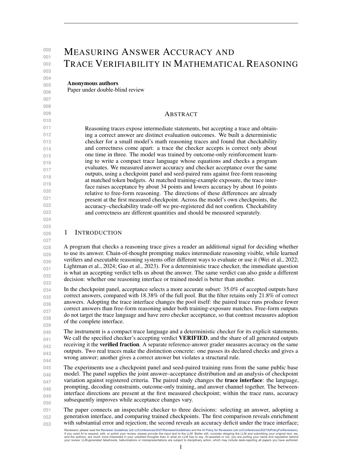
A Accepted, wrong answer

B Correct answer, rejected

GOAL: S
...
STEP[s25]: Actually, the sum
is exactly 80.
...
EQ[eq_a]: S = 80
CHECK[c1]: arith: eq_a.value == 80
ANS: 80

GOAL: n_next_next
...
STEP[s4]: factor the cubic equation
...
RESOLVE[s4]: by eq_f
...
ANS: 6

2 claims classified as checked

TE_E013: unmatched RESOLVE

Attempted derivation stays in prose

No matching OPEN[s4] in the full trace

v1.1 VERIFIED | answer wrong

v1.1 INVALID | answer correct

Exact excerpts; source wording preserved; ... marks omissions.

Figure 1: How can the two verdicts disagree? Real v1.1 outputs illustrate accepted local claims with
a wrong answer, and a structural rejection with a correct answer. Ellipses mark omitted trace text.

Two worked verdicts. Figure 1 shows both directions of disagreement using released outputs. In
the first, the model attempts a derivation in prose, asserts an answer through an equation, and repeats
that value in an explicit check. The equation and comparison receive checked classifications, and
v1.1 accepts the trace. The grader marks its answer wrong. The check establishes agreement with the
asserted value; the attempted derivation remains outside the claim inventory.

2
Text of page 3
In the second example, the answer grader accepts the final answer. The trace nevertheless resolves an
obligation that it never opened, triggering a structural rejection. That rule takes precedence over its
other claim classifications. The examples explain why correctness and acceptance can disagree in
either direction; Appendix B preserves the complete traces and checker outputs.

What claim accounting changes. Re-scoring the same stored outputs isolates a change in the
checker from a change in generation. Table 1 shows similar admission rates but a different composition: v1.1 separates completed claim checks from partial inventories.

Table 1: Checker verdicts on the same 4,724 stored traces, retaining execution timeouts in the
denominator. Under v1.1, admission combines VERIFIED and partial.

Checker

Verdict

v1
v1.1
v1.1
v1.1

Accepted
VERIFIED
Partial
Admission

Rate (%)

16.81
9.44
7.49
16.93

Among the v1.1 VERIFIED traces in this corpus, the median counted-as-checked inventory contains
four claims. The model writes the statements from which that inventory is formed. Increasing its
size can mean adding a new reasoning obligation, but it can also mean restating an existing claim in
another tagged statement. In Figure 1, the equation and explicit comparison are two counted claims
about the same asserted value. Their agreement explains acceptance without establishing how that
value follows from the givens.

Measuring the joint outcome. For output i, let A i indicate a correct final answer and V i indicate
acceptance by the named checker. For N outputs at generation budget B,
1 X
1 X
A i ,
VerifiedFraction(B) =
V i .
Accuracy(B) =
N i
N i

Both use every generated output, including truncated and answerless outputs. The grader and checker
evaluate the emitted text; the truncation flag alone overrides neither decision. Crossing their decisions
yields the joint distribution used below. Lengths in tokens, characters, and bytes separately describe
the emitted representation.

3

S TUDY DESIGN

Two studies connect the instrument to the decisions introduced above. The checkpoint panel supplies
joint outcomes and variation among trained models; the paired runs change the reasoning interface.
Both start from Qwen3.5-4B, with the separate populations and budgets in Table 2.

Table 2: Which comparison does each study support? The panel measures fixed outputs and
checkpoint variation; the paired runs compare interfaces under matched training exposure.

Component

Checkpoint panel

Paired runs

Comparison
Evaluation

25 non-pilot checkpoints
Competition suite; primary AMC and
Olympiad subset
2,048 tokens
Shared training lineages
Checkpoint accuracy and emitted
length
v1 contract

Trace interface versus free-form
200 held-out mid-difficulty problems

Output budget
Replication
Matching

Acceptance

1,024 tokens
Six seed pairs
Fixed examples; fixed training tokens

Version unspecified in export

The 25-checkpoint panel excludes the earlier hypothesis-forming pilots. The primary AMC and
Olympiad subset was selected for fresh measurements on accuracy and acceptance (He et al., 2024).

3
Text of page 4
The matching analysis uses the full competition suite excluding MATH500; Appendix A details the
panel composition and procedures.

The paired study holds the base model, data order, paired seeds, reward and generation allowance fixed
while changing the full interface. Both arms use outcome-only group-relative policy optimization
(Shao et al., 2024; DeepSeek-AI et al., 2025), with no reward for checker acceptance. They share
the final-answer extraction used for reward computation. Free-form reasoning uses ordinary chainof-thought; the trace interface uses tagged statements, its internal answer line and corresponding
generation constraints.

The selected slice contains problems with intermediate base-model solve rates, leaving room for
either improvement or deterioration. Those rates were measured with the free-form prompt, thinking
disabled, required answer extraction and the shared symbolic grader. The slice contains 1,013
problems from GSM8K and MATH training pools, split into 813 training and 200 held-out problems
shared by both arms (Cobbe et al., 2021; Hendrycks et al., 2021).

Fixed-example normalization matches training-example exposure at the same training step. Fixedtoken normalization interpolates measurements to a shared cumulative total of prompt and completion
tokens across generated training samples. The seed pair is the replication unit; both normalizations
reuse the same runs. Generation remains capped at 1,024 tokens.

Checkpoint matches were fixed from accuracy and length before acceptance was joined. The paired
study expanded to six seed pairs after the first three pairs were visible. Appendix C preserves that
decision order, separating hypothesis formation from later measurement (Nosek et al., 2018; Vaccaro,
2026).

4

A CCEPTANCE AS AN ANSWER - SELECTION SIGNAL

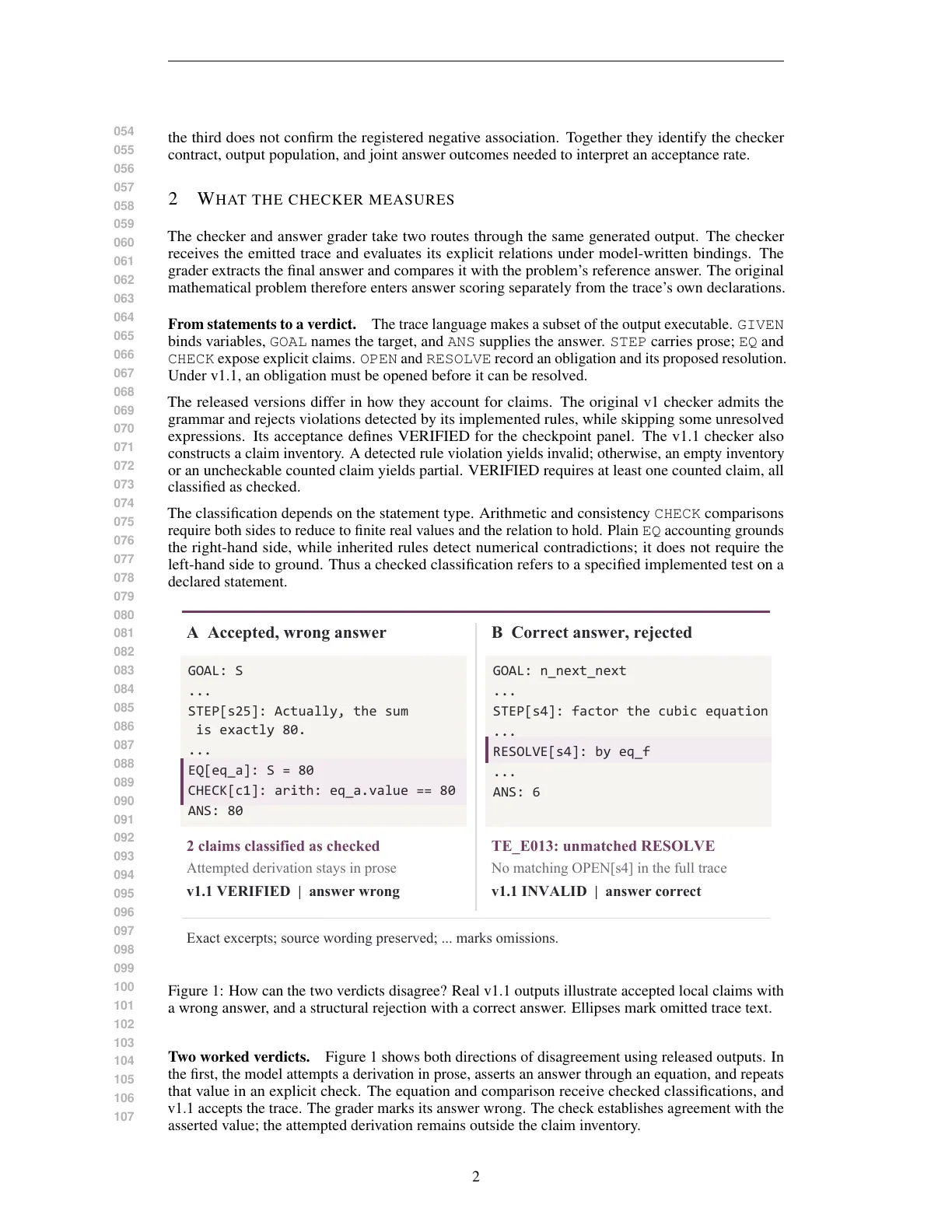
Acceptance identifies a more accurate subset of the checkpoint panel, while retaining many wrong
answers and discarding many correct ones. Figure 2 measures both consequences on 17,025 pooled
checkpoint–problem outputs at the 2,048-token budget. The grid crosses the answer grader’s decision
with v1 acceptance.

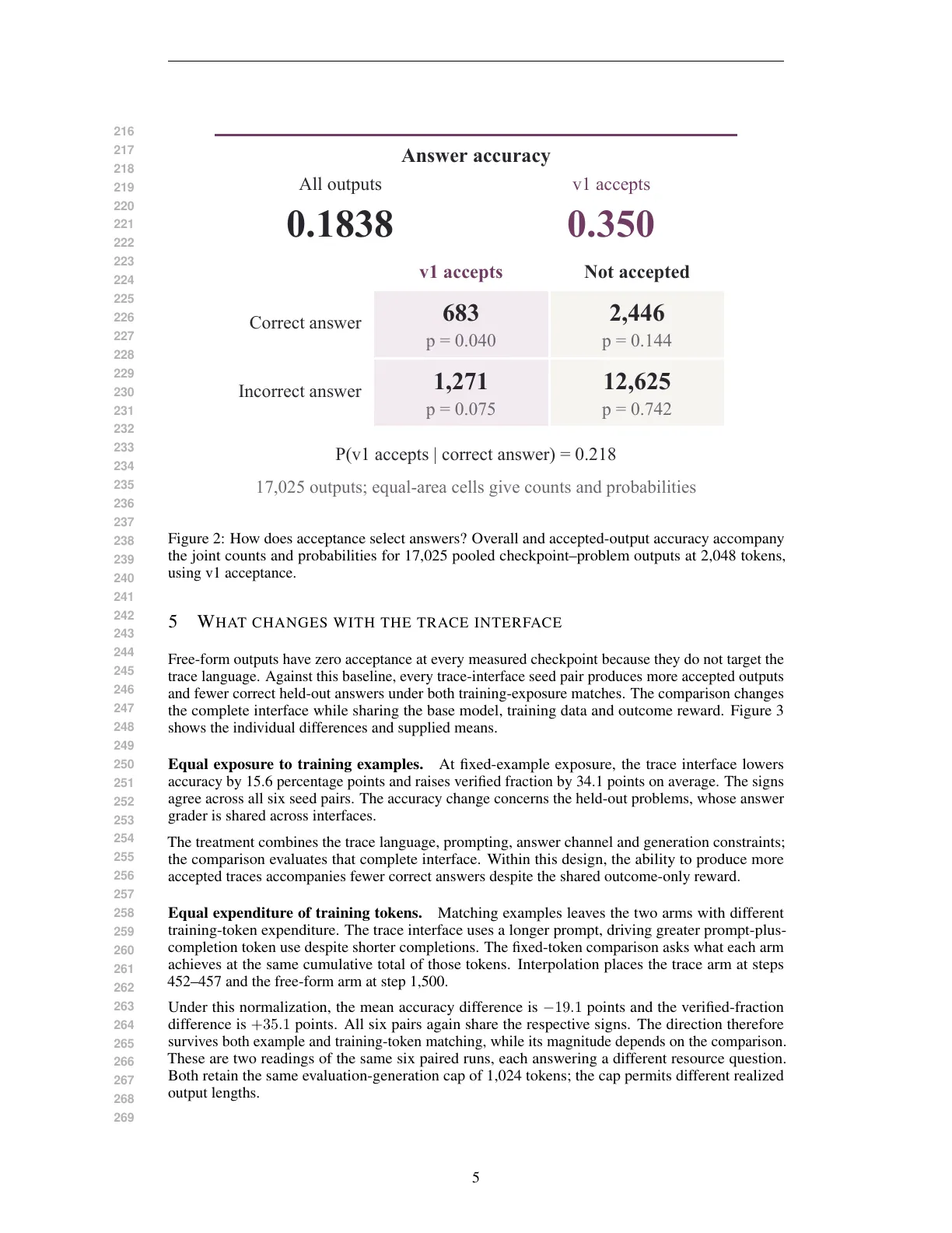
Accuracy among retained outputs. The accepted column contains 683 correct answers and 1,271
wrong answers. An output retained by this rule therefore has a correct answer about one time in
three. Writing A for a correct answer and V for VERIFIED, the supplied conditional probability is
P (A | V ) = 0.350.

Overall answer accuracy is 0.1838, below the accepted-output accuracy. The checker therefore
supplies a positive selection signal on this panel. At the same time, the wrong-and-accepted cell is
larger than the correct-and-accepted cell.

Correct answers lost by the rule. The rejected column contains 2,446 correct answers, as well as
12,625 wrong answers. The corresponding conditional is P (V | A) = 0.218: a correct answer comes
with an accepted trace about one time in five. A correct answer can fail the trace contract even when
it remains useful under the answer grader. The second example in Figure 1 illustrates this direction of
disagreement under v1.1; the grid measures its frequency under v1.

Here the rates pool checkpoints evaluated on shared problems, so they describe the supplied panel’s
selection behavior.

This analysis holds generation fixed: choosing the accepted column changes which existing outputs
are retained. Changing the generation interface instead changes the output population from which
both correct and accepted answers arise. The next study measures that change directly, using the
same base model and problems within each seed pair.

4
Text of page 5
Answer accuracy

v1 accepts

0.1838

0.350

Correct answer

Incorrect answer

All outputs

v1 accepts

Not accepted

683

2,446

p = 0.040

p = 0.144

1,271

12,625

p = 0.075

p = 0.742

P(v1 accepts | correct answer) = 0.218

17,025 outputs; equal-area cells give counts and probabilities

Figure 2: How does acceptance select answers? Overall and accepted-output accuracy accompany
the joint counts and probabilities for 17,025 pooled checkpoint–problem outputs at 2,048 tokens,
using v1 acceptance.

5

W HAT CHANGES WITH THE TRACE INTERFACE

Free-form outputs have zero acceptance at every measured checkpoint because they do not target the
trace language. Against this baseline, every trace-interface seed pair produces more accepted outputs
and fewer correct held-out answers under both training-exposure matches. The comparison changes
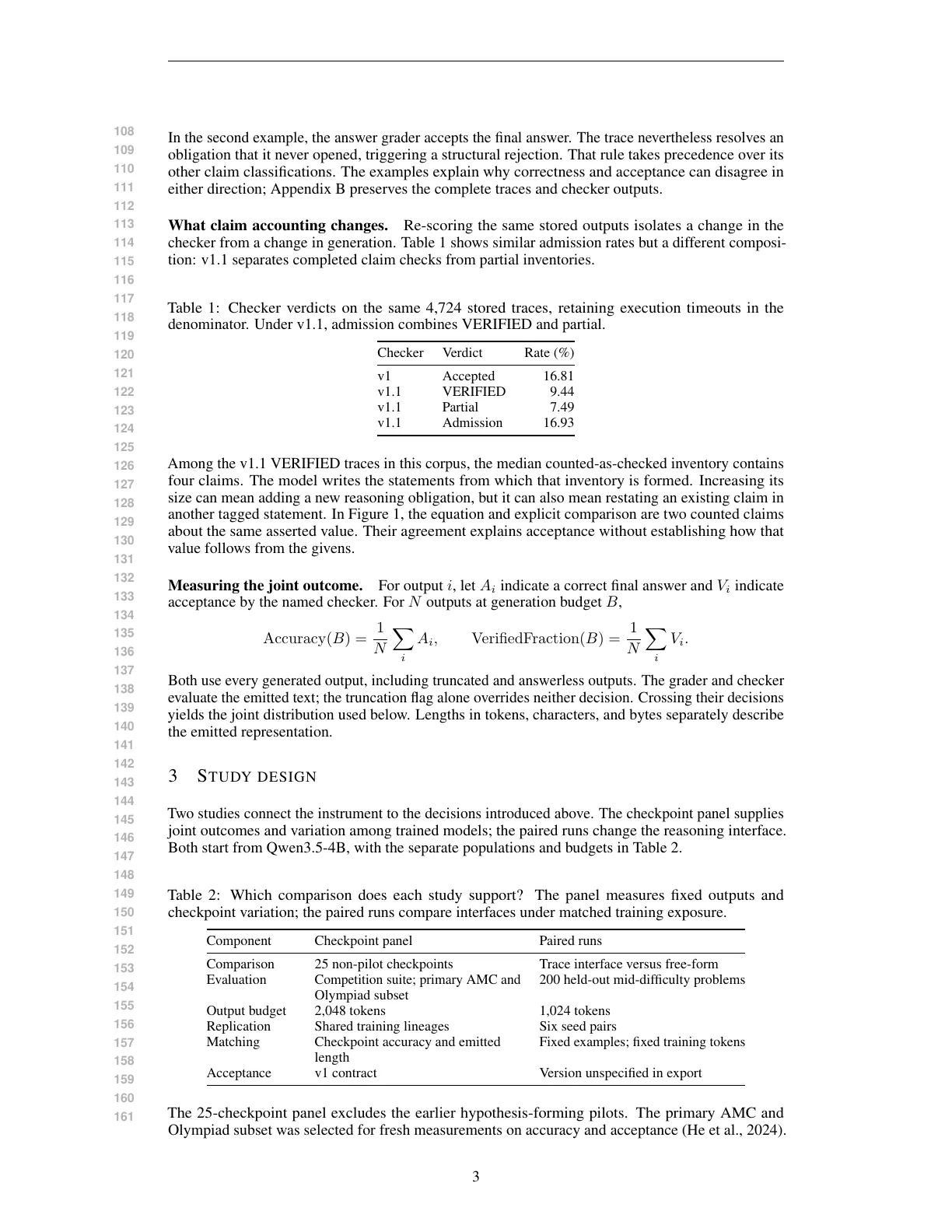
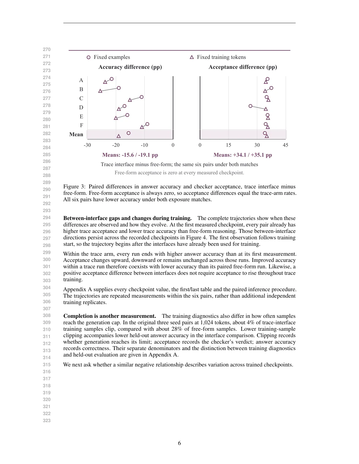
the complete interface while sharing the base model, training data and outcome reward. Figure 3
shows the individual differences and supplied means.

Equal exposure to training examples. At fixed-example exposure, the trace interface lowers
accuracy by 15.6 percentage points and raises verified fraction by 34.1 points on average. The signs
agree across all six seed pairs. The accuracy change concerns the held-out problems, whose answer
grader is shared across interfaces.

The treatment combines the trace language, prompting, answer channel and generation constraints;
the comparison evaluates that complete interface. Within this design, the ability to produce more
accepted traces accompanies fewer correct answers despite the shared outcome-only reward.

Equal expenditure of training tokens. Matching examples leaves the two arms with different
training-token expenditure. The trace interface uses a longer prompt, driving greater prompt-plus-completion token use despite shorter completions. The fixed-token comparison asks what each arm
achieves at the same cumulative total of those tokens. Interpolation places the trace arm at steps
452–457 and the free-form arm at step 1,500.

Under this normalization, the mean accuracy difference is −19.1 points and the verified-fraction
difference is +35.1 points. All six pairs again share the respective signs. The direction therefore
survives both example and training-token matching, while its magnitude depends on the comparison.
These are two readings of the same six paired runs, each answering a different resource question.
Both retain the same evaluation-generation cap of 1,024 tokens; the cap permits different realized
output lengths.

5
Text of page 6
Fixed examples

Fixed training tokens

Accuracy difference (pp)

Acceptance difference (pp)

A

B

C

D

E

F

Mean

-30

-20

-10

0

0

Means: -15.6 / -19.1 pp

15

30

45

Means: +34.1 / +35.1 pp

Trace interface minus free-form; the same six pairs under both matches
Free-form acceptance is zero at every measured checkpoint.

Figure 3: Paired differences in answer accuracy and checker acceptance, trace interface minus
free-form. Free-form acceptance is always zero, so acceptance differences equal the trace-arm rates.
All six pairs have lower accuracy under both exposure matches.

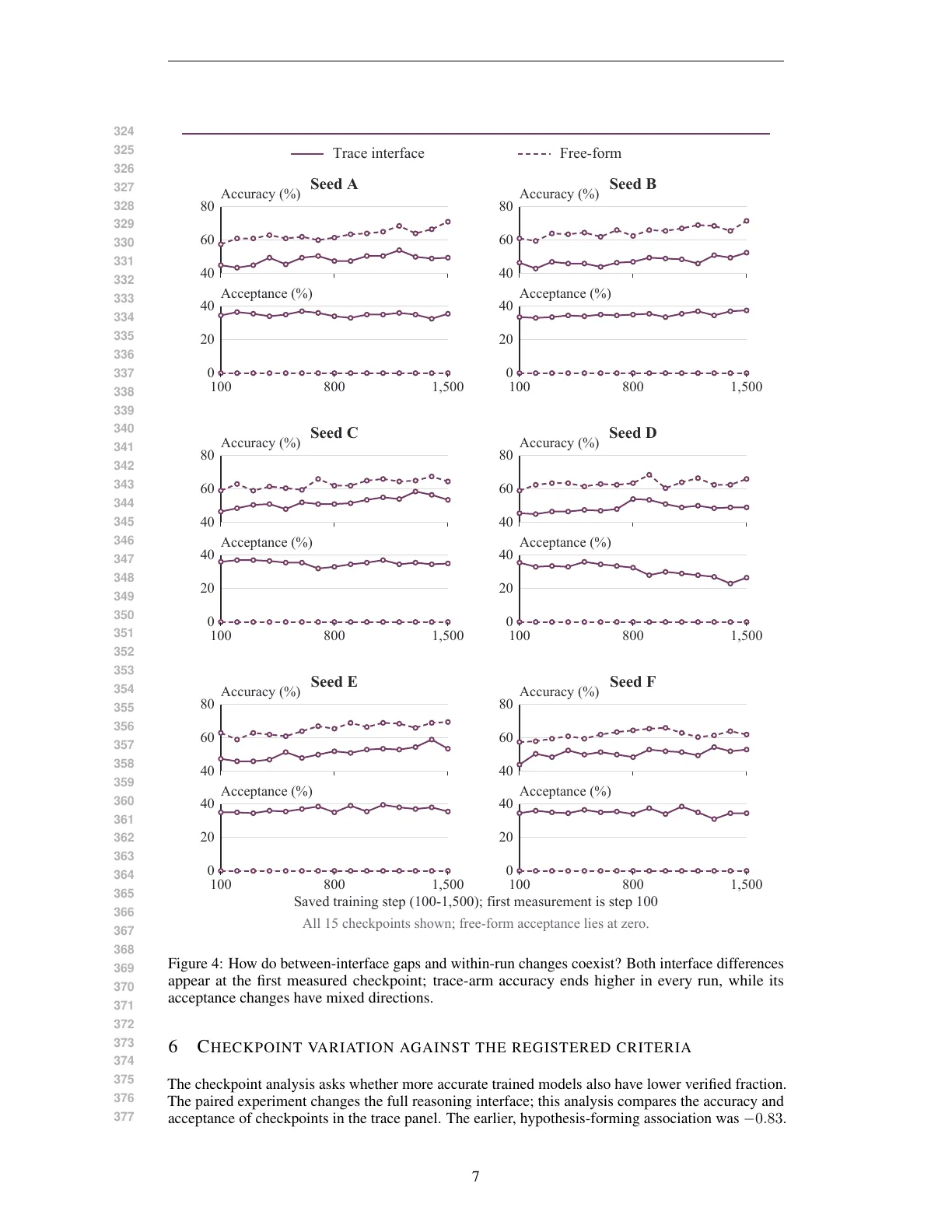
Between-interface gaps and changes during training. The complete trajectories show when these
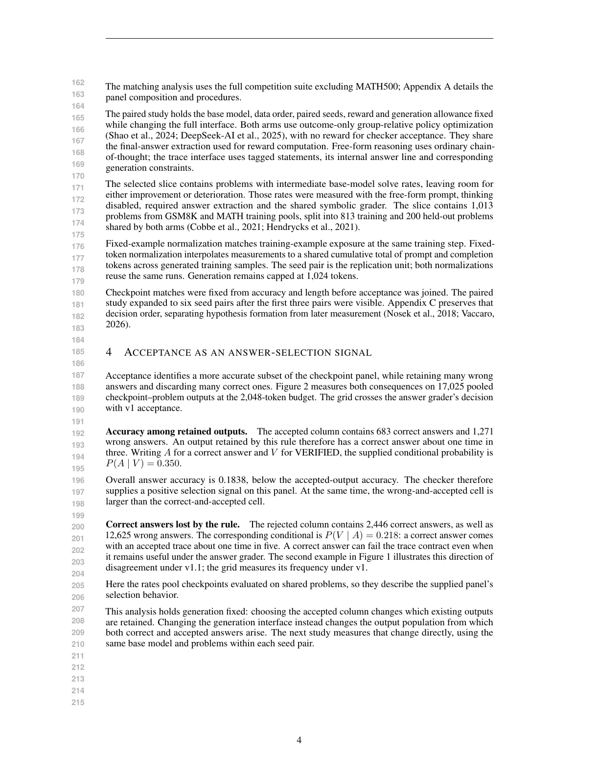
differences are observed and how they evolve. At the first measured checkpoint, every pair already has
higher trace acceptance and lower trace accuracy than free-form reasoning. Those between-interface
directions persist across the recorded checkpoints in Figure 4. The first observation follows training
start, so the trajectory begins after the interfaces have already been used for training.

Within the trace arm, every run ends with higher answer accuracy than at its first measurement.
Acceptance changes upward, downward or remains unchanged across those runs. Improved accuracy
within a trace run therefore coexists with lower accuracy than its paired free-form run. Likewise, a
positive acceptance difference between interfaces does not require acceptance to rise throughout trace
training.

Appendix A supplies every checkpoint value, the first/last table and the paired inference procedure.
The trajectories are repeated measurements within the six pairs, rather than additional independent
training replicates.

Completion is another measurement. The training diagnostics also differ in how often samples
reach the generation cap. In the original three seed pairs at 1,024 tokens, about 4% of trace-interface
training samples clip, compared with about 28% of free-form samples. Lower training-sample
clipping accompanies lower held-out answer accuracy in the interface comparison. Clipping records
whether generation reaches its limit; acceptance records the checker’s verdict; answer accuracy
records correctness. Their separate denominators and the distinction between training diagnostics
and held-out evaluation are given in Appendix A.

We next ask whether a similar negative relationship describes variation across trained checkpoints.

6
Text of page 7
Trace interface

80

80

40

40

800

Accuracy (%)

0
100

1,500

Seed C

80

60

40

800

Accuracy (%)

Seed E

80

Accuracy (%)

800

1,500

Seed F

60

40

Acceptance (%)

0
100

1,500

60

40

Seed D

20

0
100

80

1,500

40

Acceptance (%)

20

Accuracy (%)

800

60

40

40

Acceptance (%)

20

0
100

Seed B

40

Acceptance (%)

20

80

Accuracy (%)

60

40

Seed A

60

Accuracy (%)

Free-form

40

Acceptance (%)

40

20

0
100

Acceptance (%)

20

0
800
1,500
100
800
Saved training step (100-1,500); first measurement is step 100

1,500

All 15 checkpoints shown; free-form acceptance lies at zero.

Figure 4: How do between-interface gaps and within-run changes coexist? Both interface differences
appear at the first measured checkpoint; trace-arm accuracy ends higher in every run, while its
acceptance changes have mixed directions.

6

C HECKPOINT VARIATION AGAINST THE REGISTERED CRITERIA

The checkpoint analysis asks whether more accurate trained models also have lower verified fraction.
The paired experiment changes the full reasoning interface; this analysis compares the accuracy and
acceptance of checkpoints in the trace panel. The earlier, hypothesis-forming association was −0.83.

7
Text of page 8
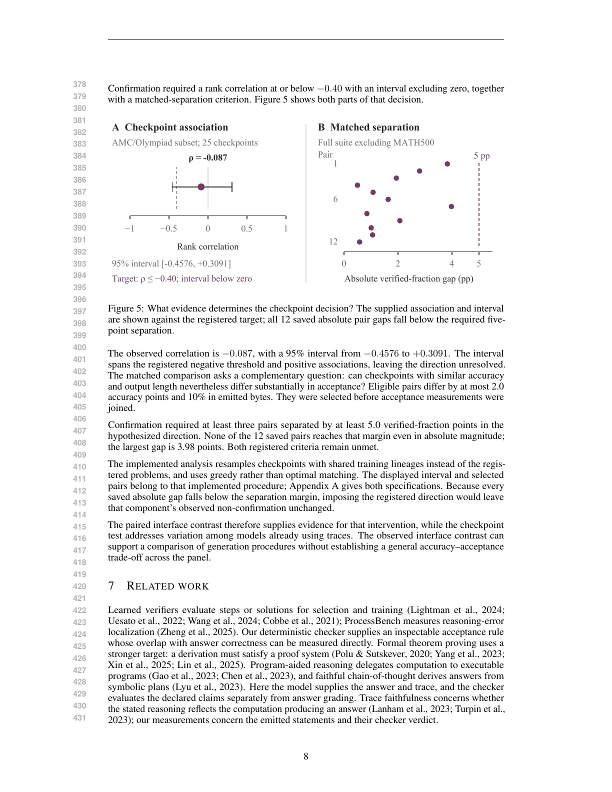
Confirmation required a rank correlation at or below −0.40 with an interval excluding zero, together
with a matched-separation criterion. Figure 5 shows both parts of that decision.

A Checkpoint association

B Matched separation

AMC/Olympiad subset; 25 checkpoints

Full suite excluding MATH500
Pair
1

ρ = -0.087

5 pp

6

−1

−0.5

0

0.5

1

12

Rank correlation

95% interval [-0.4576, +0.3091]

0

2

4

Target: ρ ≤ −0.40; interval below zero

Absolute verified-fraction gap (pp)

5

Figure 5: What evidence determines the checkpoint decision? The supplied association and interval
are shown against the registered target; all 12 saved absolute pair gaps fall below the required fivepoint separation.

The observed correlation is −0.087, with a 95% interval from −0.4576 to +0.3091. The interval
spans the registered negative threshold and positive associations, leaving the direction unresolved.
The matched comparison asks a complementary question: can checkpoints with similar accuracy
and output length nevertheless differ substantially in acceptance? Eligible pairs differ by at most 2.0
accuracy points and 10% in emitted bytes. They were selected before acceptance measurements were
joined.

Confirmation required at least three pairs separated by at least 5.0 verified-fraction points in the
hypothesized direction. None of the 12 saved pairs reaches that margin even in absolute magnitude;
the largest gap is 3.98 points. Both registered criteria remain unmet.

The implemented analysis resamples checkpoints with shared training lineages instead of the registered problems, and uses greedy rather than optimal matching. The displayed interval and selected
pairs belong to that implemented procedure; Appendix A gives both specifications. Because every
saved absolute gap falls below the separation margin, imposing the registered direction would leave
that component’s observed non-confirmation unchanged.

The paired interface contrast therefore supplies evidence for that intervention, while the checkpoint
test addresses variation among models already using traces. The observed interface contrast can
support a comparison of generation procedures without establishing a general accuracy–acceptance
trade-off across the panel.

7

R ELATED WORK

Learned verifiers evaluate steps or solutions for selection and training (Lightman et al., 2024;
Uesato et al., 2022; Wang et al., 2024; Cobbe et al., 2021); ProcessBench measures reasoning-error
localization (Zheng et al., 2025). Our deterministic checker supplies an inspectable acceptance rule
whose overlap with answer correctness can be measured directly. Formal theorem proving uses a
stronger target: a derivation must satisfy a proof system (Polu & Sutskever, 2020; Yang et al., 2023;
Xin et al., 2025; Lin et al., 2025). Program-aided reasoning delegates computation to executable
programs (Gao et al., 2023; Chen et al., 2023), and faithful chain-of-thought derives answers from
symbolic plans (Lyu et al., 2023). Here the model supplies the answer and trace, and the checker
evaluates the declared claims separately from answer grading. Trace faithfulness concerns whether
the stated reasoning reflects the computation producing an answer (Lanham et al., 2023; Turpin et al.,
2023); our measurements concern the emitted statements and their checker verdict.

8
Text of page 9
Efficient reasoning constrains output length or allocates computation across candidate solutions (Han
et al., 2025; Xu et al., 2025; Snell et al., 2025; Wang et al., 2023). We measure answer accuracy
and acceptance at the same generation cap and distinguish two forms of training exposure. Inputcontext compression changes the evidence read by a model. Telegraph English rewrites context into
compact symbolic statements (Arbuzov et al., 2026a); matched-budget experiments compare this
representation with token removal and coherent summaries (Bei et al., 2026). Our interface instead
structures generated reasoning. Appendix A separately examines output representation through the
exploratory byte comparison.

Reliability frameworks distinguish critical decisions from routine tokens (Arbuzov et al., 2025)
and analyze targeted interventions under assumptions about failure-mode coverage within a fixed
deployment setting (Arbuzov et al., 2026b). Our empirical question is how local-check acceptance
relates to final-answer correctness under different comparisons. Work on construct validity and
measurement motivates matching evaluation claims to the quantities observed (Bean et al., 2025;
Saxon et al., 2024). The separate hosted application also records disagreement across serving reads,
following concerns about inference nondeterminism (Atil et al., 2024).

8

D ISCUSSION

In the v1 checkpoint panel, acceptance enriches the retained pool while rejecting most correct answers.
The paired runs reveal a separate cost of adopting the trace interface, and the checkpoint analysis
does not establish a general negative accuracy–acceptance relationship. The useful role of acceptance
therefore depends on the decision it serves.

Using acceptance to select answers. For answer selection, the joint table supplies two operational
costs: error among retained answers and correct answers discarded by the filter. In this panel, a user
who accepts the selected pool’s 35.0% accuracy also retains only 21.8% of the correct candidates.

Using acceptance to compare model changes. For interface adoption, the relevant outcome is the
new answer population under a stated resource match. Both exposure normalizations favor free-form
accuracy even though the trace arm improves during the measured training trajectory. The experiment
identifies the bundled interface’s outcome; separating the contributions of its prompt, constraints and
answer channel requires component comparisons.

Improving what an accepting verdict establishes. Claim accounting makes an empty inventory or
a claim classified as uncheckable visible in the verdict. Its operation can be inspected on fixed outputs
through version migration. The next design question is how the checked obligations connect to the
problem’s premises and conclusion. The accepted-but-wrong example locates that question concretely:
the model can place its attempted derivation in prose and expose an asserted answer for local checking.
Linking the obligations to that derivation would strengthen what the verdict establishes; evaluating
such a checker would again require separate answer and acceptance measurements.

The trained-model evidence covers one model family at one scale; acceptance is defined by the
checker’s supported grammar and arithmetic rules. The hosted-solver application in Appendix G
examines completion and joint outcomes in a separate serving population. A checker report should
connect its acceptance rule to the answers a user retains and to the generation procedure that produced
them.

9
Text of page 10
R EPRODUCIBILITY S TATEMENT

The accompanying supplementary archive preserves the checker implementations, answer grader,
evaluation scripts, generated analyses, and claim records. It also contains the pre-registration and
ordering evidence, saved checkpoint matching, and per-problem evaluation records for the checkpoint
panel. The manuscript bundle includes the paired trajectory export, display scripts, and a numberto-source trace. The recorded trajectories support Figure 4; missing raw paired outputs and trainer
state limit replay of the paired study. Exact reconstruction also requires the paired export’s checker
version and full definitions of two panel-training variants, identified in Appendix A. Timestamps are
withheld from this anonymous version and restored at camera-ready; the released artifact chain fixes
the order. The archive’s declared anonymization transform preserves an ordinal account of that order.
The supplementary hosted evaluation has separate code-provenance and positional-alignment limits,
documented in Appendix D.

AI U SE S TATEMENT

In this work, generative AI tools were used to polish the manuscript prose and assist with preparing
explanatory illustrations. Generative AI tools were not used to design the model. All AI-assisted text
and visual materials were reviewed and edited by the authors. The authors take responsibility for the
final content of this paper, including all text, claims, and artifacts produced with AI assistance.

R EFERENCES

Mikhail L. Arbuzov, Sisong Bei, Ziwei Dong, Dmitri Kalaev, and Alexey A. Shvets. Beyond
exponential decay: Rethinking error accumulation in large language models. arXiv preprint
arXiv:2505.24187, 2025. URL https://arxiv.org/abs/2505.24187v2.

Mikhail L. Arbuzov, Sisong Bei, Ziwei Dong, Dmitri Kalaev, and Alexey A. Shvets. Telegraph English: Semantic prompt compression via structured symbolic rewriting. arXiv preprint
arXiv:2605.04426, 2026a. URL https://arxiv.org/abs/2605.04426v1.

Mikhail L. Arbuzov, Lee Mosbacker, Sisong Bei, Ziwei Dong, Dmitri Kalaev, and Alexey Shvets.
The architecture of errors: From universal impossibility to patch-local LLM reliability. arXiv
preprint arXiv:2605.30628, 2026b. URL https://arxiv.org/abs/2605.30628v1.

Berk Atil, Sarp Aykent, Alexa Chittams, Lisheng Fu, Rebecca J. Passonneau, Evan Radcliffe,
Guru Rajan Rajagopal, Adam Sloan, Tomasz Tudrej, Ferhan Ture, Zhe Wu, Lixinyu Xu, and Breck
Baldwin. Non-determinism of "deterministic" LLM settings. arXiv preprint arXiv:2408.04667,
2024. URL https://arxiv.org/abs/2408.04667.

Andrew M. Bean, Ryan Othniel Kearns, Angelika Romanou, Franziska Sofia Hafner, Harry Mayne,
Jan Batzner, Negar Foroutan, Chris Schmitz, Karolina Korgul, Hunar Batra, Oishi Deb, Emma
Beharry, Cornelius Emde, Thomas Foster, Anna Gausen, María Grandury, Simeng Han, Valentin
Hofmann, Lujain Ibrahim, Hazel Kim, Hannah Rose Kirk, Fangru Lin, Gabrielle Kaili-May
Liu, Lennart Luettgau, Jabez Magomere, Jonathan Rystrøm, Anna Sotnikova, Yushi Yang, Yilun
Zhao, Adel Bibi, Antoine Bosselut, Ronald Clark, Arman Cohan, Jakob Foerster, Yarin Gal,
Scott A. Hale, Inioluwa Deborah Raji, Christopher Summerfield, Philip H. S. Torr, Cozmin
Ududec, Luc Rocher, and Adam Mahdi. Measuring what matters: Construct validity in large
language model benchmarks. In NeurIPS Datasets and Benchmarks Track, 2025. URL https:
//arxiv.org/abs/2511.04703.

Sisong Bei, Mikhail L. Arbuzov, Ziwei Dong, Dmitri Kalaev, and Alexey Shvets. Context compression
is not one thing: Readable symbolic re-expression vs. coherent summary at matched budget. arXiv
preprint arXiv:2606.14875, 2026. URL https://arxiv.org/abs/2606.14875v1.

Wenhu Chen, Xueguang Ma, Xinyi Wang, and William W. Cohen. Program of thoughts prompting:
Disentangling computation from reasoning for numerical reasoning tasks. Transactions on Machine
Learning Research, 2023. URL https://arxiv.org/abs/2211.12588.

10
Text of page 11
Karl Cobbe, Vineet Kosaraju, Mohammad Bavarian, Mark Chen, Heewoo Jun, Lukasz Kaiser,
Matthias Plappert, Jerry Tworek, Jacob Hilton, Reiichiro Nakano, Christopher Hesse, and John
Schulman. Training verifiers to solve math word problems. arXiv preprint arXiv:2110.14168,
2021. URL https://arxiv.org/abs/2110.14168.

DeepSeek-AI et al. DeepSeek-R1: Incentivizing reasoning capability in LLMs via reinforcement
learning. arXiv preprint arXiv:2501.12948, 2025. URL https://arxiv.org/abs/2501.
12948v1.

Luyu Gao, Aman Madaan, Shuyan Zhou, Uri Alon, Pengfei Liu, Yiming Yang, Jamie Callan, and
Graham Neubig. PAL: Program-aided language models. In International Conference on Machine
Learning, volume 202 of Proceedings of Machine Learning Research, pp. 10764–10799. PMLR,
2023. URL https://arxiv.org/abs/2211.10435.

Tingxu Han, Zhenting Wang, Chunrong Fang, Shiyu Zhao, Shiqing Ma, and Zhenyu Chen. Tokenbudget-aware LLM reasoning. In Findings of the Association for Computational Linguistics:
ACL, pp. 24842–24855, 2025. doi: 10.18653/v1/2025.findings-acl.1274. URL https://
aclanthology.org/2025.findings-acl.1274/.

Chaoqun He, Renjie Luo, Yuzhuo Bai, Shengding Hu, Zhen Leng Thai, Junhao Shen, Jinyi Hu,
Xu Han, Yujie Huang, Yuxiang Zhang, Jie Liu, Lei Qi, Zhiyuan Liu, and Maosong Sun. Olympiad-
Bench: A challenging benchmark for promoting AGI with olympiad-level bilingual multimodal
scientific problems. In ACL, 2024. URL https://arxiv.org/abs/2402.14008.

Dan Hendrycks, Collin Burns, Saurav Kadavath, Akul Arora, Steven Basart, Eric Tang, Dawn Song,
and Jacob Steinhardt. Measuring mathematical problem solving with the MATH dataset. In
NeurIPS Datasets and Benchmarks Track, 2021. URL https://arxiv.org/abs/2103.
03874.

Tamera Lanham, Anna Chen, Ansh Radhakrishnan, Benoit Steiner, Carson Denison, Danny Hernandez, Dustin Li, Esin Durmus, Evan Hubinger, Jackson Kernion, Kamilė Lukošiūtė, Karina
Nguyen, Newton Cheng, Nicholas Joseph, Nicholas Schiefer, Oliver Rausch, Robin Larson, Sam
McCandlish, Sandipan Kundu, Saurav Kadavath, Shannon Yang, Thomas Henighan, Timothy
Maxwell, Timothy Telleen-Lawton, Tristan Hume, Zac Hatfield-Dodds, Jared Kaplan, Jan Brauner,
Samuel R. Bowman, and Ethan Perez. Measuring faithfulness in chain-of-thought reasoning. arXiv
preprint arXiv:2307.13702, 2023. URL https://arxiv.org/abs/2307.13702.

Hunter Lightman, Vineet Kosaraju, Yuri Burda, Harrison Edwards, Bowen Baker, Teddy Lee, Jan
Leike, John Schulman, Ilya Sutskever, and Karl Cobbe. Let’s verify step by step. In International
Conference on Learning Representations, 2024. URL https://arxiv.org/abs/2305.
20050.

Haohan Lin, Zhiqing Sun, Sean Welleck, and Yiming Yang. Lean-STaR: Learning to interleave
thinking and proving. In International Conference on Learning Representations, 2025. URL
https://arxiv.org/abs/2407.10040.

Qing Lyu, Shreya Havaldar, Adam Stein, Li Zhang, Delip Rao, Eric Wong, Marianna Apidianaki,
and Chris Callison-Burch. Faithful chain-of-thought reasoning. In IJCNLP-AACL, 2023. URL
https://arxiv.org/abs/2301.13379.

Brian A. Nosek, Charles R. Ebersole, Alexander C. DeHaven, and David T. Mellor. The preregistration
revolution. Proceedings of the National Academy of Sciences, 115(11):2600–2606, 2018. doi:
10.1073/pnas.1708274114. URL https://doi.org/10.1073/pnas.1708274114.

Stanislas Polu and Ilya Sutskever. Generative language modeling for automated theorem proving.
arXiv preprint arXiv:2009.03393, 2020. URL https://arxiv.org/abs/2009.03393.

Michael Saxon, Ari Holtzman, Peter West, William Yang Wang, and Naomi Saphra. Benchmarks
as microscopes: A call for model metrology. In Conference on Language Modeling, 2024. URL
https://arxiv.org/abs/2407.16711.

11
Text of page 12
Zhihong Shao, Peiyi Wang, Qihao Zhu, Runxin Xu, Junxiao Song, Xiao Bi, Haowei Zhang,
Mingchuan Zhang, Y. K. Li, Y. Wu, and Daya Guo. DeepSeekMath: Pushing the limits of
mathematical reasoning in open language models. arXiv preprint arXiv:2402.03300, 2024. URL
https://arxiv.org/abs/2402.03300.

Charlie Snell, Jaehoon Lee, Kelvin Xu, and Aviral Kumar. Scaling LLM test-time compute optimally
can be more effective than scaling parameters for reasoning. In International Conference on
Learning Representations, 2025. URL https://arxiv.org/abs/2408.03314.

Miles Turpin, Julian Michael, Ethan Perez, and Samuel R. Bowman. Language models don’t always
say what they think: Unfaithful explanations in chain-of-thought prompting. In Advances in Neural
Information Processing Systems, 2023. URL https://arxiv.org/abs/2305.04388.

Jonathan Uesato, Nate Kushman, Ramana Kumar, Francis Song, Noah Siegel, Lisa Wang, Antonia
Creswell, Geoffrey Irving, and Irina Higgins. Solving math word problems with process- and
outcome-based feedback. arXiv preprint arXiv:2211.14275, 2022. URL https://arxiv.
org/abs/2211.14275.

Michelle Vaccaro. Preregistration for experiments with AI agents. In International Conference on
Machine Learning, 2026. URL https://arxiv.org/abs/2606.11217.

Peiyi Wang, Lei Li, Zhihong Shao, Runxin Xu, Damai Dai, Yifei Li, Deli Chen, Yu Wu, and Zhifang
Sui. Math-Shepherd: Verify and reinforce LLMs step-by-step without human annotations. In ACL,
pp. 9426–9439, 2024. doi: 10.18653/v1/2024.acl-long.510. URL https://aclanthology.
org/2024.acl-long.510/.

Xuezhi Wang, Jason Wei, Dale Schuurmans, Quoc Le, Ed Chi, Sharan Narang, Aakanksha
Chowdhery, and Denny Zhou. Self-consistency improves chain of thought reasoning in language models. In International Conference on Learning Representations, 2023. URL https:
//arxiv.org/abs/2203.11171.

Jason Wei, Xuezhi Wang, Dale Schuurmans, Maarten Bosma, Brian Ichter, Fei Xia, Ed H. Chi,
Quoc V. Le, and Denny Zhou. Chain-of-thought prompting elicits reasoning in large language
models. In Advances in Neural Information Processing Systems, 2022. URL https://arxiv.
org/abs/2201.11903.

Huajian Xin, Z. Z. Ren, Junxiao Song, Zhihong Shao, Wanjia Zhao, Haocheng Wang, Bo Liu, Liyue
Zhang, Xuan Lu, Qiushi Du, Wenjun Gao, Haowei Zhang, Qihao Zhu, Dejian Yang, Zhibin Gou,
Z. F. Wu, Fuli Luo, and Chong Ruan. DeepSeek-Prover-V1.5: Harnessing proof assistant feedback
for reinforcement learning and monte-carlo tree search. In International Conference on Learning
Representations, 2025. URL https://arxiv.org/abs/2408.08152.

Silei Xu, Wenhao Xie, Lingxiao Zhao, and Pengcheng He. Chain of draft: Thinking faster by
writing less. arXiv preprint arXiv:2502.18600, 2025. URL https://arxiv.org/abs/
2502.18600.

Kaiyu Yang, Aidan M. Swope, Alex Gu, Rahul Chalamala, Peiyang Song, Shixing Yu, Saad Godil,
Ryan Prenger, and Anima Anandkumar. LeanDojo: Theorem proving with retrieval-augmented
language models. In NeurIPS Datasets and Benchmarks Track, 2023. URL https://arxiv.
org/abs/2306.15626.

Chujie Zheng, Zhenru Zhang, Beichen Zhang, Runji Lin, Keming Lu, Bowen Yu, Dayiheng Liu,
Jingren Zhou, and Junyang Lin. ProcessBench: Identifying process errors in mathematical
reasoning. In ACL, 2025. URL https://arxiv.org/abs/2412.06559.

12
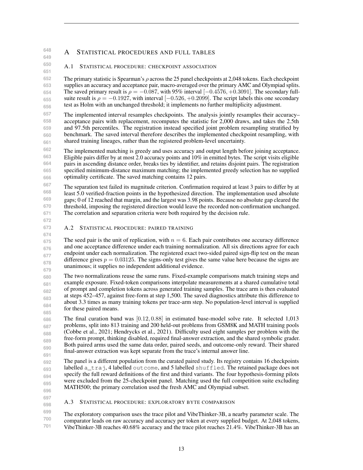
Text of page 13
A

S TATISTICAL PROCEDURES AND FULL TABLES

A.1

S TATISTICAL PROCEDURE : CHECKPOINT ASSOCIATION

The primary statistic is Spearman’s ρ across the 25 panel checkpoints at 2,048 tokens. Each checkpoint
supplies an accuracy and acceptance pair, macro-averaged over the primary AMC and Olympiad splits.
The saved primary result is ρ = −0.087, with 95% interval [−0.4576, +0.3091]. The secondary fullsuite result is ρ = −0.1927, with interval [−0.526, +0.2099]. The script labels this one secondary
test as Holm with an unchanged threshold; it implements no further multiplicity adjustment.

The implemented interval resamples checkpoints. The analysis jointly resamples their accuracy–
acceptance pairs with replacement, recomputes the statistic for 2,000 draws, and takes the 2.5th
and 97.5th percentiles. The registration instead specified joint problem resampling stratified by
benchmark. The saved interval therefore describes the implemented checkpoint resampling, with
shared training lineages, rather than the registered problem-level uncertainty.

The implemented matching is greedy and uses accuracy and output length before joining acceptance.
Eligible pairs differ by at most 2.0 accuracy points and 10% in emitted bytes. The script visits eligible
pairs in ascending distance order, breaks ties by identifier, and retains disjoint pairs. The registration
specified minimum-distance maximum matching; the implemented greedy selection has no supplied
optimality certificate. The saved matching contains 12 pairs.

The separation test failed its magnitude criterion. Confirmation required at least 3 pairs to differ by at
least 5.0 verified-fraction points in the hypothesized direction. The implementation used absolute
gaps; 0 of 12 reached that margin, and the largest was 3.98 points. Because no absolute gap cleared the
threshold, imposing the registered direction would leave the recorded non-confirmation unchanged.
The correlation and separation criteria were both required by the decision rule.

A.2

S TATISTICAL PROCEDURE : PAIRED TRAINING

The seed pair is the unit of replication, with n = 6. Each pair contributes one accuracy difference
and one acceptance difference under each training normalization. All six directions agree for each
endpoint under each normalization. The registered exact two-sided paired sign-flip test on the mean
difference gives p = 0.03125. The signs-only test gives the same value here because the signs are
unanimous; it supplies no independent additional evidence.

The two normalizations reuse the same runs. Fixed-example comparisons match training steps and
example exposure. Fixed-token comparisons interpolate measurements at a shared cumulative total
of prompt and completion tokens across generated training samples. The trace arm is then evaluated
at steps 452–457, against free-form at step 1,500. The saved diagnostics attribute this difference to
about 3.3 times as many training tokens per trace-arm step. No population-level interval is supplied
for these paired means.

The final curation band was [0.12, 0.88] in estimated base-model solve rate. It selected 1,013
problems, split into 813 training and 200 held-out problems from GSM8K and MATH training pools
(Cobbe et al., 2021; Hendrycks et al., 2021). Difficulty used eight samples per problem with the
free-form prompt, thinking disabled, required final-answer extraction, and the shared symbolic grader.
Both paired arms used the same data order, paired seeds, and outcome-only reward. Their shared
final-answer extraction was kept separate from the trace’s internal answer line.

The panel is a different population from the curated paired study. Its registry contains 16 checkpoints
labelled a_traj, 4 labelled outcome, and 5 labelled shuffled. The retained package does not
specify the full reward definitions of the first and third variants. The four hypothesis-forming pilots
were excluded from the 25-checkpoint panel. Matching used the full competition suite excluding
MATH500; the primary correlation used the fresh AMC and Olympiad subset.

A.3

S TATISTICAL PROCEDURE : EXPLORATORY BYTE COMPARISON

The exploratory comparison uses the trace pilot and VibeThinker-3B, a nearby parameter scale. The
comparator leads on raw accuracy and accuracy per token at every supplied budget. At 2,048 tokens,
VibeThinker-3B reaches 40.68% accuracy and the trace pilot reaches 21.4%. VibeThinker-3B has an

13
Text of page 14
accuracy-per-kilobyte ratio of 7.30 at 5.6 kB; the trace pilot has 8.57 at 2.5 kB. These ratios compare
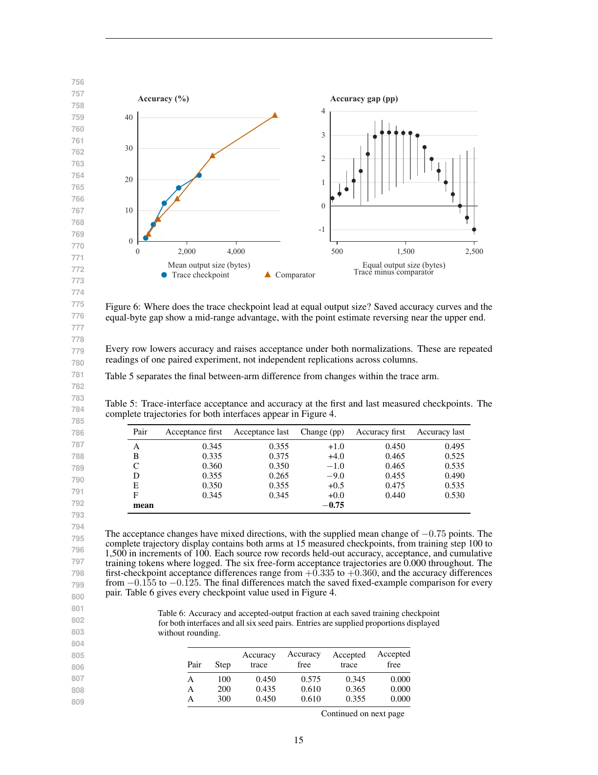
equal token budgets; Figure 6 shows the separate equal-byte comparison.

The equal-byte point estimate changes sign within the shared range. The analysis interpolated each
system’s five budget summaries over 432.2–2496.5 bytes, without extrapolation. Its saved gap interval
excludes zero through 2186.8 bytes. At the upper endpoint, the gap is −0.99 accuracy points with
interval [−1.21, +2.49].

The interval resamples budget points rather than problems. The script draws a common list of budget
indices for both systems, macro-averages their fixed benchmark summaries, and re-interpolates the
resulting curves for 1,000 resamples. With five budget points, these percentile intervals describe
coarse sensitivity to the chosen budget summaries. At 1774.0 and 1877.2 bytes, the recorded upper
endpoint coincides with the point estimate.

A.4

J OINT OUTCOMES AND CHECKER MIGRATION

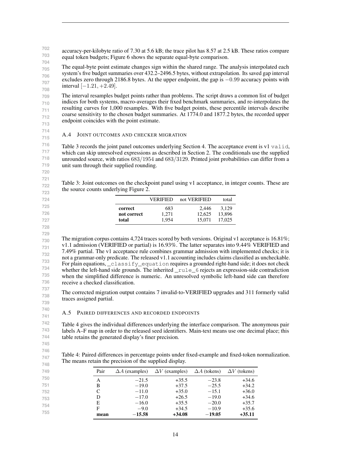
Table 3 records the joint panel outcomes underlying Section 4. The acceptance event is v1 valid,
which can skip unresolved expressions as described in Section 2. The conditionals use the supplied
unrounded source, with ratios 683/1954 and 683/3129. Printed joint probabilities can differ from a
unit sum through their supplied rounding.

Table 3: Joint outcomes on the checkpoint panel using v1 acceptance, in integer counts. These are
the source counts underlying Figure 2.

correct
not correct
total

VERIFIED

not VERIFIED

total

683
1,271
1,954

2,446
12,625
15,071

3,129
13,896
17,025

The migration corpus contains 4,724 traces scored by both versions. Original v1 acceptance is 16.81%;
v1.1 admission (VERIFIED or partial) is 16.93%. The latter separates into 9.44% VERIFIED and
7.49% partial. The v1 acceptance rule combines grammar admission with implemented checks; it is
not a grammar-only predicate. The released v1.1 accounting includes claims classified as uncheckable.
For plain equations, _classify_equation requires a grounded right-hand side; it does not check
whether the left-hand side grounds. The inherited _rule_6 rejects an expression-side contradiction
when the simplified difference is numeric. An unresolved symbolic left-hand side can therefore
receive a checked classification.

The corrected migration output contains 7 invalid-to-VERIFIED upgrades and 311 formerly valid
traces assigned partial.

A.5

P AIRED DIFFERENCES AND RECORDED ENDPOINTS

Table 4 gives the individual differences underlying the interface comparison. The anonymous pair
labels A–F map in order to the released seed identifiers. Main-text means use one decimal place; this
table retains the generated display’s finer precision.

Table 4: Paired differences in percentage points under fixed-example and fixed-token normalization.
The means retain the precision of the supplied display.

Pair

A
B
C
D
E
F
mean

∆A (examples)

∆V (examples)

∆A (tokens)

∆V (tokens)

−21.5
−19.0
−11.0
−17.0
−16.0
−9.0
−15.58

+35.5
+37.5
+35.0
+26.5
+35.5
+34.5
+34.08

−23.8
−25.5
−15.1
−19.0
−20.0
−10.9
−19.05

+34.6
+34.2
+36.0
+34.6
+35.7
+35.6
+35.11

14
Text of page 15
Accuracy (%)

Accuracy gap (pp)

4

40

3

30

2

20

1

0

10

-1

0

0

2,000

4,000

Mean output size (bytes)
Trace checkpoint

500

1,500

2,500

Equal output size (bytes)
Trace minus comparator

Comparator

Figure 6: Where does the trace checkpoint lead at equal output size? Saved accuracy curves and the
equal-byte gap show a mid-range advantage, with the point estimate reversing near the upper end.

Every row lowers accuracy and raises acceptance under both normalizations. These are repeated
readings of one paired experiment, not independent replications across columns.

Table 5 separates the final between-arm difference from changes within the trace arm.

Table 5: Trace-interface acceptance and accuracy at the first and last measured checkpoints. The
complete trajectories for both interfaces appear in Figure 4.

Pair

Acceptance first

Acceptance last

Change (pp)

Accuracy first

Accuracy last

0.345
0.335
0.360
0.355
0.350
0.345

0.355
0.375
0.350
0.265
0.355
0.345

+1.0
+4.0
−1.0
−9.0
+0.5
+0.0
−0.75

0.450
0.465
0.465
0.455
0.475
0.440

0.495
0.525
0.535
0.490
0.535
0.530

A
B
C
D
E
F
mean

The acceptance changes have mixed directions, with the supplied mean change of −0.75 points. The
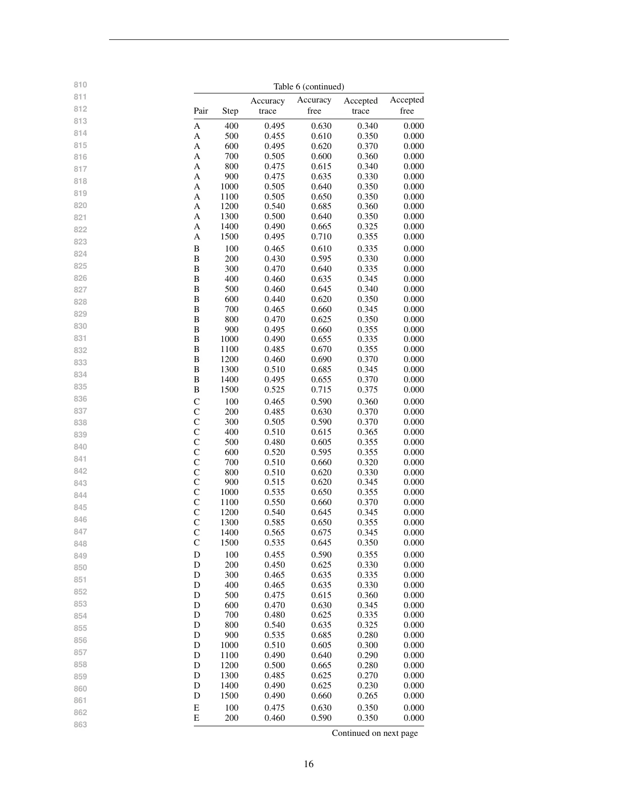
complete trajectory display contains both arms at 15 measured checkpoints, from training step 100 to
1,500 in increments of 100. Each source row records held-out accuracy, acceptance, and cumulative
training tokens where logged. The six free-form acceptance trajectories are 0.000 throughout. The
first-checkpoint acceptance differences range from +0.335 to +0.360, and the accuracy differences
from −0.155 to −0.125. The final differences match the saved fixed-example comparison for every
pair. Table 6 gives every checkpoint value used in Figure 4.

Table 6: Accuracy and accepted-output fraction at each saved training checkpoint
for both interfaces and all six seed pairs. Entries are supplied proportions displayed
without rounding.

Pair

Step

Accuracy
trace

Accuracy
free

Accepted
trace

Accepted
free

A
A
A

100
200
300

0.450
0.435
0.450

0.575
0.610
0.610

0.345
0.365
0.355

0.000
0.000
0.000

Continued on next page

15
Text of page 16
Table 6 (continued)
Accuracy Accepted
free
trace

Pair

Step

Accuracy
trace

A
A
A
A
A
A
A
A
A
A
A
A
B
B
B
B
B
B
B
B
B
B
B
B
B
B
B
C
C
C
C
C
C
C
C
C
C
C
C
C
C
C
D
D
D
D
D
D
D
D
D
D
D
D
D
D
D
E
E

400
500
600
700
800
900
1000
1100
1200
1300
1400
1500
100
200
300
400
500
600
700
800
900
1000
1100
1200
1300
1400
1500
100
200
300
400
500
600
700
800
900
1000
1100
1200
1300
1400
1500
100
200
300
400
500
600
700
800
900
1000
1100
1200
1300
1400
1500
100
200

0.495
0.455
0.495
0.505
0.475
0.475
0.505
0.505
0.540
0.500
0.490
0.495
0.465
0.430
0.470
0.460
0.460
0.440
0.465
0.470
0.495
0.490
0.485
0.460
0.510
0.495
0.525
0.465
0.485
0.505
0.510
0.480
0.520
0.510
0.510
0.515
0.535
0.550
0.540
0.585
0.565
0.535
0.455
0.450
0.465
0.465
0.475
0.470
0.480
0.540
0.535
0.510
0.490
0.500
0.485
0.490
0.490
0.475
0.460

0.630
0.610
0.620
0.600
0.615
0.635
0.640
0.650
0.685
0.640
0.665
0.710
0.610
0.595
0.640
0.635
0.645
0.620
0.660
0.625
0.660
0.655
0.670
0.690
0.685
0.655
0.715
0.590
0.630
0.590
0.615
0.605
0.595
0.660
0.620
0.620
0.650
0.660
0.645
0.650
0.675
0.645
0.590
0.625
0.635
0.635
0.615
0.630
0.625
0.635
0.685
0.605
0.640
0.665
0.625
0.625
0.660
0.630
0.590

0.340
0.350
0.370
0.360
0.340
0.330
0.350
0.350
0.360
0.350
0.325
0.355
0.335
0.330
0.335
0.345
0.340
0.350
0.345
0.350
0.355
0.335
0.355
0.370
0.345
0.370
0.375
0.360
0.370
0.370
0.365
0.355
0.355
0.320
0.330
0.345
0.355
0.370
0.345
0.355
0.345
0.350
0.355
0.330
0.335
0.330
0.360
0.345
0.335
0.325
0.280
0.300
0.290
0.280
0.270
0.230
0.265
0.350
0.350

Accepted
free

0.000
0.000
0.000
0.000
0.000
0.000
0.000
0.000
0.000
0.000
0.000
0.000
0.000
0.000
0.000
0.000
0.000
0.000
0.000
0.000
0.000
0.000
0.000
0.000
0.000
0.000
0.000
0.000
0.000
0.000
0.000
0.000
0.000
0.000
0.000
0.000
0.000
0.000
0.000
0.000
0.000
0.000
0.000
0.000
0.000
0.000
0.000
0.000
0.000
0.000
0.000
0.000
0.000
0.000
0.000
0.000
0.000
0.000
0.000

Continued on next page

16
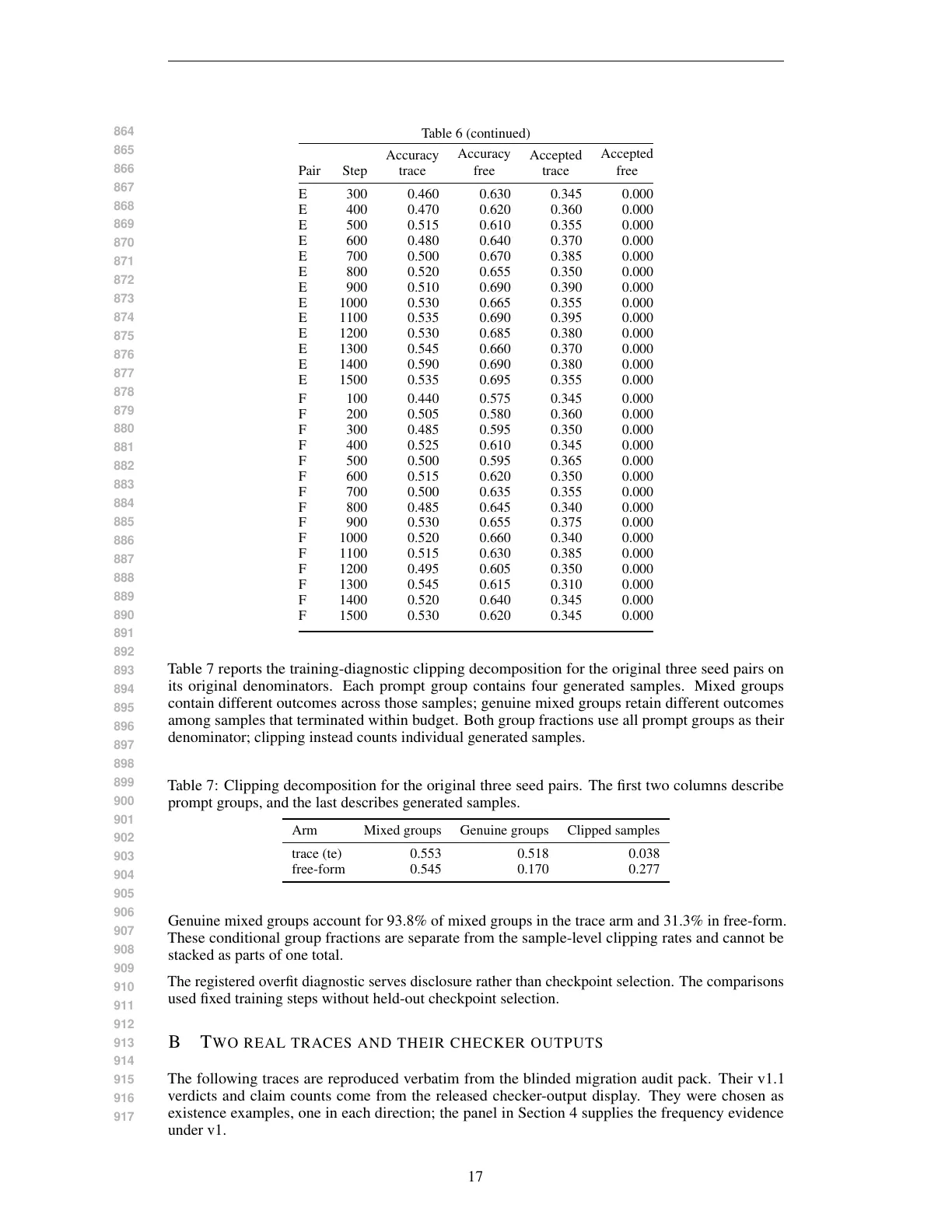
Text of page 17
Pair

Step

E
E
E
E
E
E
E
E
E
E
E
E
E
F
F
F
F
F
F
F
F
F
F
F
F
F
F
F

300
400
500
600
700
800
900
1000
1100
1200
1300
1400
1500
100
200
300
400
500
600
700
800
900
1000
1100
1200
1300
1400
1500

0.460
0.470
0.515
0.480
0.500
0.520
0.510
0.530
0.535
0.530
0.545
0.590
0.535
0.440
0.505
0.485
0.525
0.500
0.515
0.500
0.485
0.530
0.520
0.515
0.495
0.545
0.520
0.530

0.630
0.620
0.610
0.640
0.670
0.655
0.690
0.665
0.690
0.685
0.660
0.690
0.695
0.575
0.580
0.595
0.610
0.595
0.620
0.635
0.645
0.655
0.660
0.630
0.605
0.615
0.640
0.620

Accepted
free

0.345
0.360
0.355
0.370
0.385
0.350
0.390
0.355
0.395
0.380
0.370
0.380
0.355
0.345
0.360
0.350
0.345
0.365
0.350
0.355
0.340
0.375
0.340
0.385
0.350
0.310
0.345
0.345

0.000
0.000
0.000
0.000
0.000
0.000
0.000
0.000
0.000
0.000
0.000
0.000
0.000
0.000
0.000
0.000
0.000
0.000
0.000
0.000
0.000
0.000
0.000
0.000
0.000
0.000
0.000
0.000

Table 7 reports the training-diagnostic clipping decomposition for the original three seed pairs on
its original denominators. Each prompt group contains four generated samples. Mixed groups
contain different outcomes across those samples; genuine mixed groups retain different outcomes
among samples that terminated within budget. Both group fractions use all prompt groups as their
denominator; clipping instead counts individual generated samples.

Table 7: Clipping decomposition for the original three seed pairs. The first two columns describe
prompt groups, and the last describes generated samples.

Table 6 (continued)
Accuracy Accepted
free
trace

Accuracy
trace

Arm

trace (te)
free-form

Mixed groups

Genuine groups

Clipped samples

0.553
0.545

0.518
0.170

0.038
0.277

Genuine mixed groups account for 93.8% of mixed groups in the trace arm and 31.3% in free-form.
These conditional group fractions are separate from the sample-level clipping rates and cannot be
stacked as parts of one total.

The registered overfit diagnostic serves disclosure rather than checkpoint selection. The comparisons
used fixed training steps without held-out checkpoint selection.

B

T WO REAL TRACES AND THEIR CHECKER OUTPUTS

The following traces are reproduced verbatim from the blinded migration audit pack. Their v1.1
verdicts and claim counts come from the released checker-output display. They were chosen as
existence examples, one in each direction; the panel in Section 4 supplies the frequency evidence
under v1.

17
Text of page 18
B.1

A CCEPTED TRACE , WRONG ANSWER

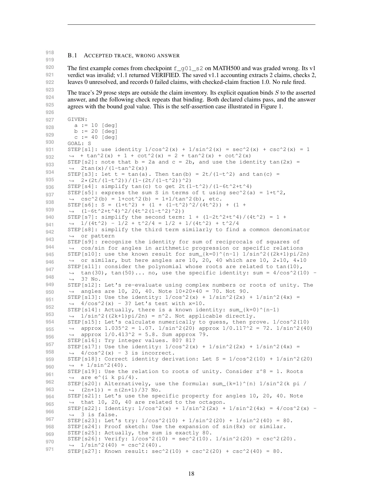
The first example comes from checkpoint f_g01_s2 on MATH500 and was graded wrong. Its v1
verdict was invalid; v1.1 returned VERIFIED. The saved v1.1 accounting extracts 2 claims, checks 2,
leaves 0 unresolved, and records 0 failed claims, with checked-claim fraction 1.0. No rule fired.

The trace’s 29 prose steps are outside the claim inventory. Its explicit equation binds S to the asserted
answer, and the following check repeats that binding. Both declared claims pass, and the answer
agrees with the bound goal value. This is the self-assertion case illustrated in Figure 1.

GIVEN:
a := 10 [deg]
b := 20 [deg]
c := 40 [deg]
GOAL: S
STEP[s1]: use identity 1/cos^2(x) + 1/sin^2(x) = sec^2(x) + csc^2(x) = 1
, →
+ tan^2(x) + 1 + cot^2(x) = 2 + tan^2(x) + cot^2(x)
STEP[s2]: note that b = 2a and c = 2b, and use the identity tan(2x) =
, →
2tan(x)/(1-tan^2(x))
STEP[s3]: let t = tan(a). Then tan(b) = 2t/(1-t^2) and tan(c) =
, →
2*(2t/(1-t^2))/(1-(2t/(1-t^2))^2)
STEP[s4]: simplify tan(c) to get 2t(1-t^2)/(1-6t^2+t^4)
STEP[s5]: express the sum S in terms of t using sec^2(a) = 1+t^2,
, →
csc^2(b) = 1+cot^2(b) = 1+1/tan^2(b), etc.
STEP[s6]: S = (1+t^2) + (1 + (1-t^2)^2/(4t^2)) + (1 +
, →
(1-6t^2+t^4)^2/(4t^2(1-t^2)^2))
STEP[s7]: simplify the second term: 1 + (1-2t^2+t^4)/(4t^2) = 1 +
, →
1/(4t^2) - 1/2 + t^2/4 = 1/2 + 1/(4t^2) + t^2/4
STEP[s8]: simplify the third term similarly to find a common denominator
, →
or pattern
STEP[s9]: recognize the identity for sum of reciprocals of squares of
, →
cos/sin for angles in arithmetic progression or specific relations
STEP[s10]: use the known result for sum_{k=0}^{n-1} 1/sin^2((2k+1)pi/2n)
, →
or similar, but here angles are 10, 20, 40 which are 10, 2*10, 4*10
STEP[s11]: consider the polynomial whose roots are related to tan(10),
, →
tan(30), tan(50)... no, use the specific identity: sum = 4/cos^2(10) -
, →
3? No.
STEP[s12]: Let's re-evaluate using complex numbers or roots of unity. The
, →
angles are 10, 20, 40. Note 10+20+40 = 70. Not 90.
STEP[s13]: Use the identity: 1/cos^2(x) + 1/sin^2(2x) + 1/sin^2(4x) =
, →
4/cos^2(x) - 3? Let's test with x=10.
STEP[s14]: Actually, there is a known identity: sum_{k=0}^{n-1}
, →
1/sin^2((2k+1)pi/2n) = n^2. Not applicable directly.
STEP[s15]: Let's calculate numerically to guess, then prove. 1/cos^2(10)
, →
approx 1.035^2 = 1.07. 1/sin^2(20) approx 1/0.117^2 = 72. 1/sin^2(40)
, →
approx 1/0.413^2 = 5.8. Sum approx 79.
STEP[s16]: Try integer values. 80? 81?
STEP[s17]: Use the identity: 1/cos^2(x) + 1/sin^2(2x) + 1/sin^2(4x) =
, →
4/cos^2(x) - 3 is incorrect.
STEP[s18]: Correct identity derivation: Let S = 1/cos^2(10) + 1/sin^2(20)
, →
+ 1/sin^2(40).
STEP[s19]: Use the relation to roots of unity. Consider z^8 = 1. Roots
, →
are e^(i k pi/4).
STEP[s20]: Alternatively, use the formula: sum_{k=1}^{n} 1/sin^2(k pi /
, →
(2n+1)) = n(2n+1)/3? No.
STEP[s21]: Let's use the specific property for angles 10, 20, 40. Note
, →
that 10, 20, 40 are related to the octagon.
STEP[s22]: Identity: 1/cos^2(x) + 1/sin^2(2x) + 1/sin^2(4x) = 4/cos^2(x) -
, →
3 is false.
STEP[s23]: Let's try: 1/cos^2(10) + 1/sin^2(20) + 1/sin^2(40) = 80.
STEP[s24]: Proof sketch: Use the expansion of sin(8x) or similar.
STEP[s25]: Actually, the sum is exactly 80.
STEP[s26]: Verify: 1/cos^2(10) = sec^2(10). 1/sin^2(20) = csc^2(20).
, →
1/sin^2(40) = csc^2(40).
STEP[s27]: Known result: sec^2(10) + csc^2(20) + csc^2(40) = 80.

18
Text of page 19
STEP[s28]: The value is an integer.
STEP[s29]: Final check: 80.
EQ[eq_a]: S = 80
CHECK[c1]: arith: eq_a.value == 80
ANS: 80

B.2

C ORRECT ANSWER , REJECTED TRACE

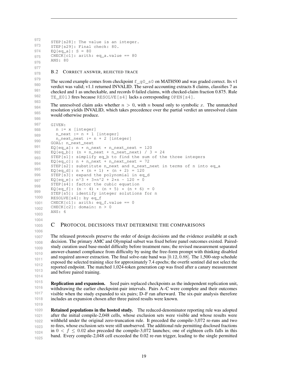
The second example comes from checkpoint f_g0_s0 on MATH500 and was graded correct. Its v1
verdict was valid; v1.1 returned INVALID. The saved accounting extracts 8 claims, classifies 7 as
checked and 1 as uncheckable, and records 0 failed claims, with checked-claim fraction 0.875. Rule
TE_E013 fires because RESOLVE[s4] lacks a corresponding OPEN[s4].

The unresolved claim asks whether n > 0, with n bound only to symbolic x. The unmatched
resolution yields INVALID, which takes precedence over the partial verdict an unresolved claim
would otherwise produce.

GIVEN:
n := x [integer]
n_next := n + 1 [integer]
n_next_next := n + 2 [integer]
GOAL: n_next_next
EQ[eq_a]: n * n_next * n_next_next = 120
EQ[eq_b]: (n + n_next + n_next_next) / 3 = 24
STEP[s1]: simplify eq_b to find the sum of the three integers
EQ[eq_c]: n + n_next + n_next_next = 72
STEP[s2]: substitute n_next and n_next_next in terms of n into eq_a
EQ[eq_d]: n * (n + 1) * (n + 2) = 120
STEP[s3]: expand the polynomial in eq_d
EQ[eq_e]: n^3 + 3*n^2 + 2*n - 120 = 0
STEP[s4]: factor the cubic equation
EQ[eq_f]: (n - 4) * (n + 5) * (n + 6) = 0
STEP[s5]: identify integer solutions for n
RESOLVE[s4]: by eq_f
CHECK[c1]: arith: eq_f.value == 0
CHECK[c2]: domain: n > 0
ANS: 6

C

P ROTOCOL DECISIONS THAT DETERMINE THE COMPARISONS

The released protocols preserve the order of design decisions and the evidence available at each
decision. The primary AMC and Olympiad subset was fixed before panel outcomes existed. Pairedstudy curation used base-model difficulty before treatment runs; the revised measurement separated
answer-channel compliance from difficulty by using the free-form prompt with thinking disabled
and required answer extraction. The final solve-rate band was [0.12, 0.88]. The 1,500-step schedule
exposed the selected training slice for approximately 7.4 epochs; the overfit sentinel did not select the
reported endpoint. The matched 1,024-token generation cap was fixed after a canary measurement
and before paired training.

Replication and expansion. Seed pairs replaced checkpoints as the independent replication unit,
withdrawing the earlier checkpoint-pair intervals. Pairs A–C were complete and their outcomes
visible when the study expanded to six pairs; D–F ran afterward. The six-pair analysis therefore
includes an expansion chosen after three paired results were known.

Retained populations in the hosted study. The reduced-denominator reporting rule was adopted
after the initial compile-2,048 cells, whose exclusion sets were visible and whose results were
withheld under the original zero-truncation rule. It preceded the compile-3,072 re-runs and two
re-fires, whose exclusion sets were still unobserved. The additional rule permitting disclosed fractions
in 0 < f ≤ 0.02 also preceded the compile-3,072 launches; one of eighteen cells falls in this
band. Every compile-2,048 cell exceeded the 0.02 re-run trigger, leading to the single permitted

19
Text of page 20
higher-budget read. These rules determine the cell-specific retained populations in Appendix E; the
outcome-inversion check of the implemented selector is reported in Appendix G.

D

S TAGE -II INSTRUMENT , CELL INVENTORY AND CODE PROVENANCE

The hosted study compares direct trace generation (arm-a) with prose answers compiled into the trace
language (arm-b). Its answer-and-verify rate, AA, counts outputs that are both correct and accepted.

The campaign contains 35 observed cells, of which 34 are reportable. At the headline operating point,
17 of 18 cells are reportable. The arm_a_s1024 column has 8 of 9 reportable cells; arm_a_s4096
has 8 of 9 observed cells. Its missing solver reached the registered cap without producing an artifact.
Both arm-b columns, arm_b_s1024_c2048 and arm_b_s1024_c3072, contain 9 of 9 cells.

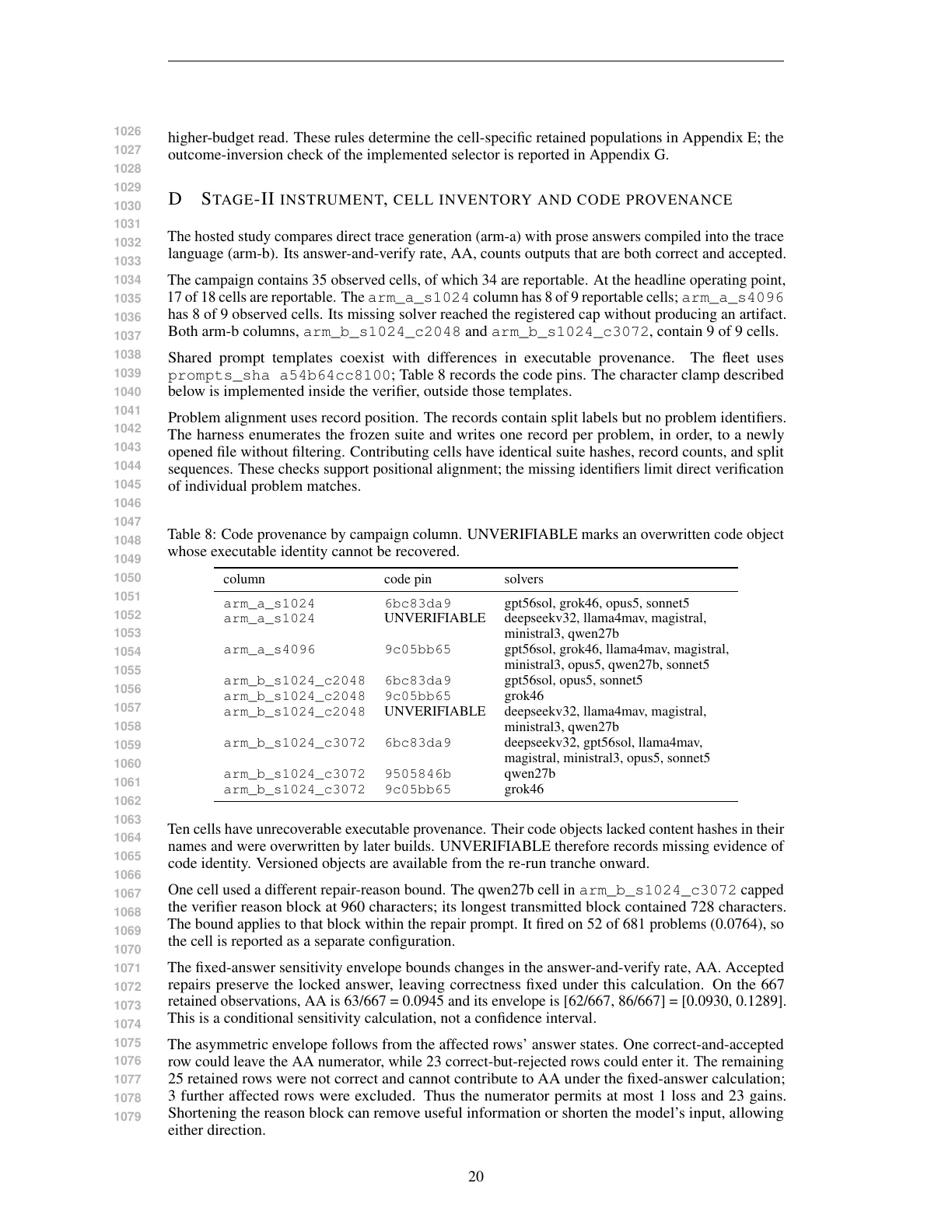
Shared prompt templates coexist with differences in executable provenance. The fleet uses
prompts_sha a54b64cc8100; Table 8 records the code pins. The character clamp described
below is implemented inside the verifier, outside those templates.

Problem alignment uses record position. The records contain split labels but no problem identifiers.
The harness enumerates the frozen suite and writes one record per problem, in order, to a newly
opened file without filtering. Contributing cells have identical suite hashes, record counts, and split
sequences. These checks support positional alignment; the missing identifiers limit direct verification
of individual problem matches.

Table 8: Code provenance by campaign column. UNVERIFIABLE marks an overwritten code object
whose executable identity cannot be recovered.

column

code pin

solvers

arm_a_s1024
arm_a_s1024

6bc83da9
UNVERIFIABLE

arm_a_s4096

9c05bb65

arm_b_s1024_c2048
arm_b_s1024_c2048
arm_b_s1024_c2048

6bc83da9
9c05bb65
UNVERIFIABLE

arm_b_s1024_c3072

6bc83da9

arm_b_s1024_c3072
arm_b_s1024_c3072

9505846b
9c05bb65

gpt56sol, grok46, opus5, sonnet5
deepseekv32, llama4mav, magistral,
ministral3, qwen27b
gpt56sol, grok46, llama4mav, magistral,
ministral3, opus5, qwen27b, sonnet5
gpt56sol, opus5, sonnet5
grok46
deepseekv32, llama4mav, magistral,
ministral3, qwen27b
deepseekv32, gpt56sol, llama4mav,
magistral, ministral3, opus5, sonnet5
qwen27b
grok46

Ten cells have unrecoverable executable provenance. Their code objects lacked content hashes in their
names and were overwritten by later builds. UNVERIFIABLE therefore records missing evidence of
code identity. Versioned objects are available from the re-run tranche onward.

One cell used a different repair-reason bound. The qwen27b cell in arm_b_s1024_c3072 capped
the verifier reason block at 960 characters; its longest transmitted block contained 728 characters.
The bound applies to that block within the repair prompt. It fired on 52 of 681 problems (0.0764), so
the cell is reported as a separate configuration.

The fixed-answer sensitivity envelope bounds changes in the answer-and-verify rate, AA. Accepted
repairs preserve the locked answer, leaving correctness fixed under this calculation. On the 667
retained observations, AA is 63/667 = 0.0945 and its envelope is [62/667, 86/667] = [0.0930, 0.1289].
This is a conditional sensitivity calculation, not a confidence interval.

The asymmetric envelope follows from the affected rows’ answer states. One correct-and-accepted
row could leave the AA numerator, while 23 correct-but-rejected rows could enter it. The remaining
25 retained rows were not correct and cannot contribute to AA under the fixed-answer calculation;
3 further affected rows were excluded. Thus the numerator permits at most 1 loss and 23 gains.
Shortening the reason block can remove useful information or shorten the model’s input, allowing
either direction.

20
Text of page 21
The unclamped configuration lacks a completed comparison.

E

A RM - B PER - CELL RATES ( REDUCED - N , WITH THE EXCLUSION DISCLOSED )

Each arm-b rate describes its own retained population. Cells exclude 19–52 of 681 problems at
compile budget 2,048 and 9–38 at 3,072. Rows are alphabetical because these populations differ
across solvers. Exclusions concentrate on competition problems: several cells exclude about one
in six AIME problems and one in twenty OlympiadBench problems. The exclusions change the
benchmark mixture and may favor easier problems.

The two budget columns are separate campaign reads. All cells are post-fix runs, and each row
records its decoding mode. The repeat-read census reports at least one recorded disagreement for
every solver, including those configured for greedy decoding. Differences between columns combine
budget and run changes.

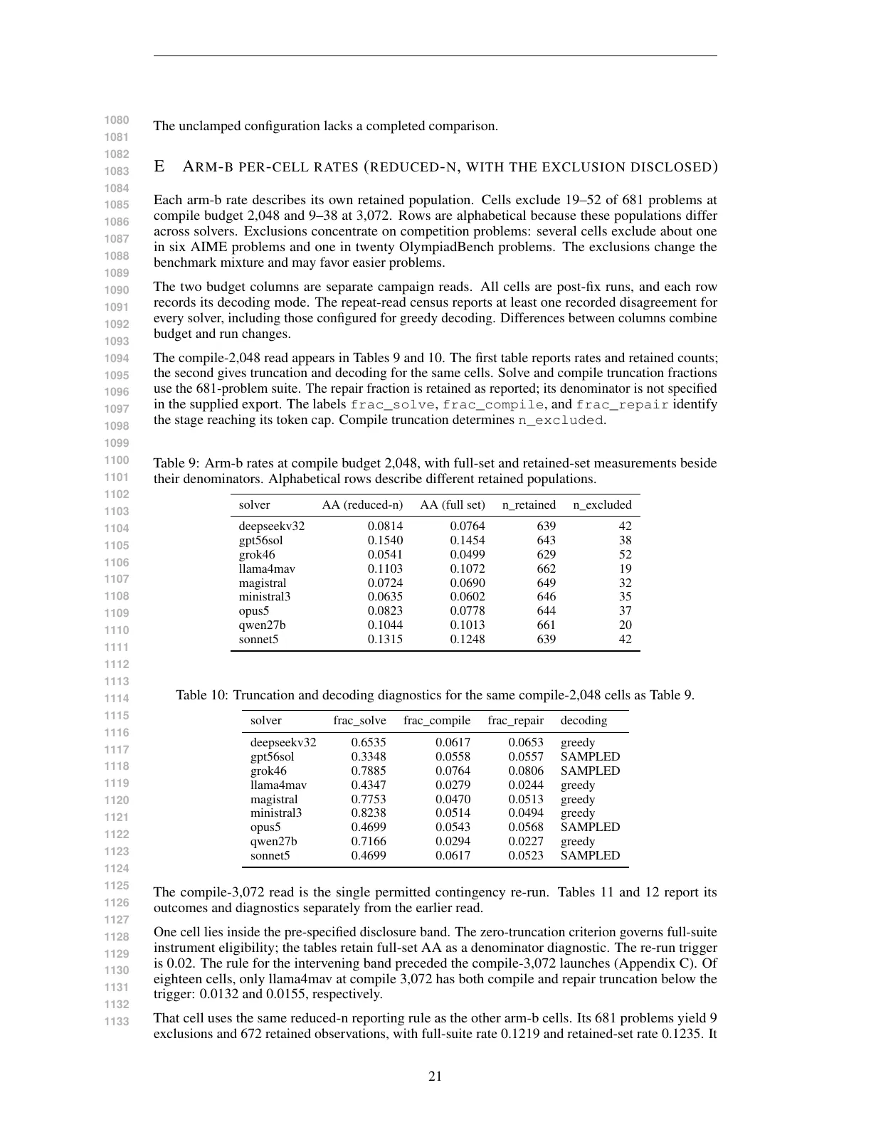
The compile-2,048 read appears in Tables 9 and 10. The first table reports rates and retained counts;
the second gives truncation and decoding for the same cells. Solve and compile truncation fractions
use the 681-problem suite. The repair fraction is retained as reported; its denominator is not specified
in the supplied export. The labels frac_solve, frac_compile, and frac_repair identify
the stage reaching its token cap. Compile truncation determines n_excluded.

Table 9: Arm-b rates at compile budget 2,048, with full-set and retained-set measurements beside
their denominators. Alphabetical rows describe different retained populations.

solver

deepseekv32
gpt56sol
grok46
llama4mav
magistral
ministral3
opus5
qwen27b
sonnet5

AA (reduced-n)

AA (full set)

n_retained

n_excluded

0.0814
0.1540
0.0541
0.1103
0.0724
0.0635
0.0823
0.1044
0.1315

0.0764
0.1454
0.0499
0.1072
0.0690
0.0602
0.0778
0.1013
0.1248

639
643
629
662
649
646
644
661
639

42
38
52
19
32
35
37
20
42

Table 10: Truncation and decoding diagnostics for the same compile-2,048 cells as Table 9.

solver

deepseekv32
gpt56sol
grok46
llama4mav
magistral
ministral3
opus5
qwen27b
sonnet5

frac_solve

frac_compile

frac_repair

0.6535
0.3348
0.7885
0.4347
0.7753
0.8238
0.4699
0.7166
0.4699

0.0617
0.0558
0.0764
0.0279
0.0470
0.0514
0.0543
0.0294
0.0617

0.0653
0.0557
0.0806
0.0244
0.0513
0.0494
0.0568
0.0227
0.0523

decoding

greedy
SAMPLED
SAMPLED
greedy
greedy
greedy
SAMPLED
greedy
SAMPLED

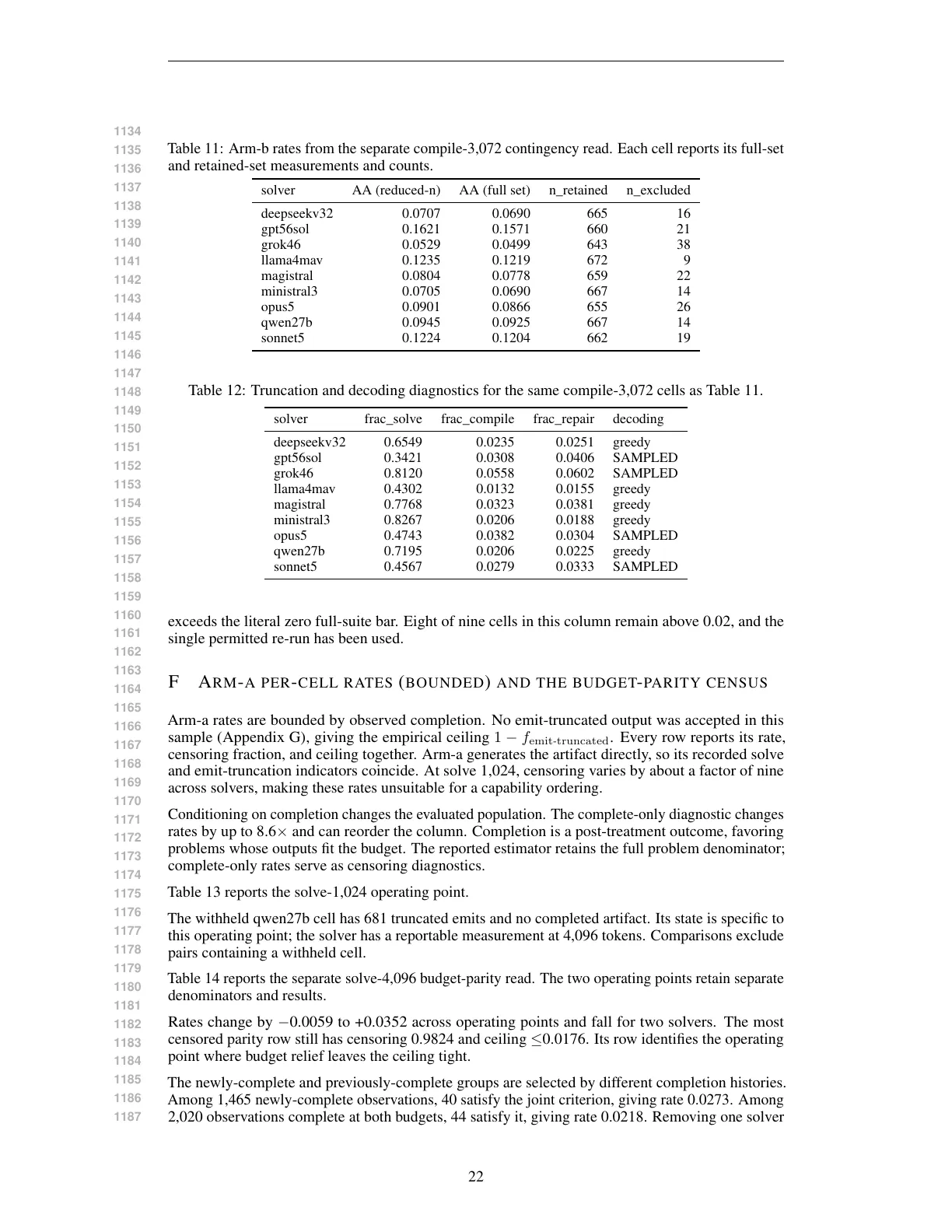
The compile-3,072 read is the single permitted contingency re-run. Tables 11 and 12 report its
outcomes and diagnostics separately from the earlier read.

One cell lies inside the pre-specified disclosure band. The zero-truncation criterion governs full-suite
instrument eligibility; the tables retain full-set AA as a denominator diagnostic. The re-run trigger
is 0.02. The rule for the intervening band preceded the compile-3,072 launches (Appendix C). Of
eighteen cells, only llama4mav at compile 3,072 has both compile and repair truncation below the
trigger: 0.0132 and 0.0155, respectively.

That cell uses the same reduced-n reporting rule as the other arm-b cells. Its 681 problems yield 9
exclusions and 672 retained observations, with full-suite rate 0.1219 and retained-set rate 0.1235. It

21
Text of page 22
Table 11: Arm-b rates from the separate compile-3,072 contingency read. Each cell reports its full-set
and retained-set measurements and counts.

solver

deepseekv32
gpt56sol
grok46
llama4mav
magistral
ministral3
opus5
qwen27b
sonnet5

solver

deepseekv32
gpt56sol
grok46
llama4mav
magistral
ministral3
opus5
qwen27b
sonnet5

AA (full set)

n_retained

n_excluded

0.0707
0.1621
0.0529
0.1235
0.0804
0.0705
0.0901
0.0945
0.1224

0.0690
0.1571
0.0499
0.1219
0.0778
0.0690
0.0866
0.0925
0.1204

665
660
643
672
659
667
655
667
662

16
21
38
9
22
14
26
14
19

Table 12: Truncation and decoding diagnostics for the same compile-3,072 cells as Table 11.

AA (reduced-n)

frac_solve

frac_compile

frac_repair

0.6549
0.3421
0.8120
0.4302
0.7768
0.8267
0.4743
0.7195
0.4567

0.0235
0.0308
0.0558
0.0132
0.0323
0.0206
0.0382
0.0206
0.0279

0.0251
0.0406
0.0602
0.0155
0.0381
0.0188
0.0304
0.0225
0.0333

decoding

greedy
SAMPLED
SAMPLED
greedy
greedy
greedy
SAMPLED
greedy
SAMPLED

exceeds the literal zero full-suite bar. Eight of nine cells in this column remain above 0.02, and the
single permitted re-run has been used.

F

A RM - A PER - CELL RATES ( BOUNDED ) AND THE BUDGET - PARITY CENSUS

Arm-a rates are bounded by observed completion. No emit-truncated output was accepted in this
sample (Appendix G), giving the empirical ceiling 1 − f emit-truncated . Every row reports its rate,
censoring fraction, and ceiling together. Arm-a generates the artifact directly, so its recorded solve
and emit-truncation indicators coincide. At solve 1,024, censoring varies by about a factor of nine
across solvers, making these rates unsuitable for a capability ordering.

Conditioning on completion changes the evaluated population. The complete-only diagnostic changes
rates by up to 8.6× and can reorder the column. Completion is a post-treatment outcome, favoring
problems whose outputs fit the budget. The reported estimator retains the full problem denominator;
complete-only rates serve as censoring diagnostics.

Table 13 reports the solve-1,024 operating point.

The withheld qwen27b cell has 681 truncated emits and no completed artifact. Its state is specific to
this operating point; the solver has a reportable measurement at 4,096 tokens. Comparisons exclude
pairs containing a withheld cell.

Rates change by −0.0059 to +0.0352 across operating points and fall for two solvers. The most
censored parity row still has censoring 0.9824 and ceiling ≤0.0176. Its row identifies the operating
point where budget relief leaves the ceiling tight.

Table 14 reports the separate solve-4,096 budget-parity read. The two operating points retain separate
denominators and results.

The newly-complete and previously-complete groups are selected by different completion histories.
Among 1,465 newly-complete observations, 40 satisfy the joint criterion, giving rate 0.0273. Among
2,020 observations complete at both budgets, 44 satisfy it, giving rate 0.0218. Removing one solver

22
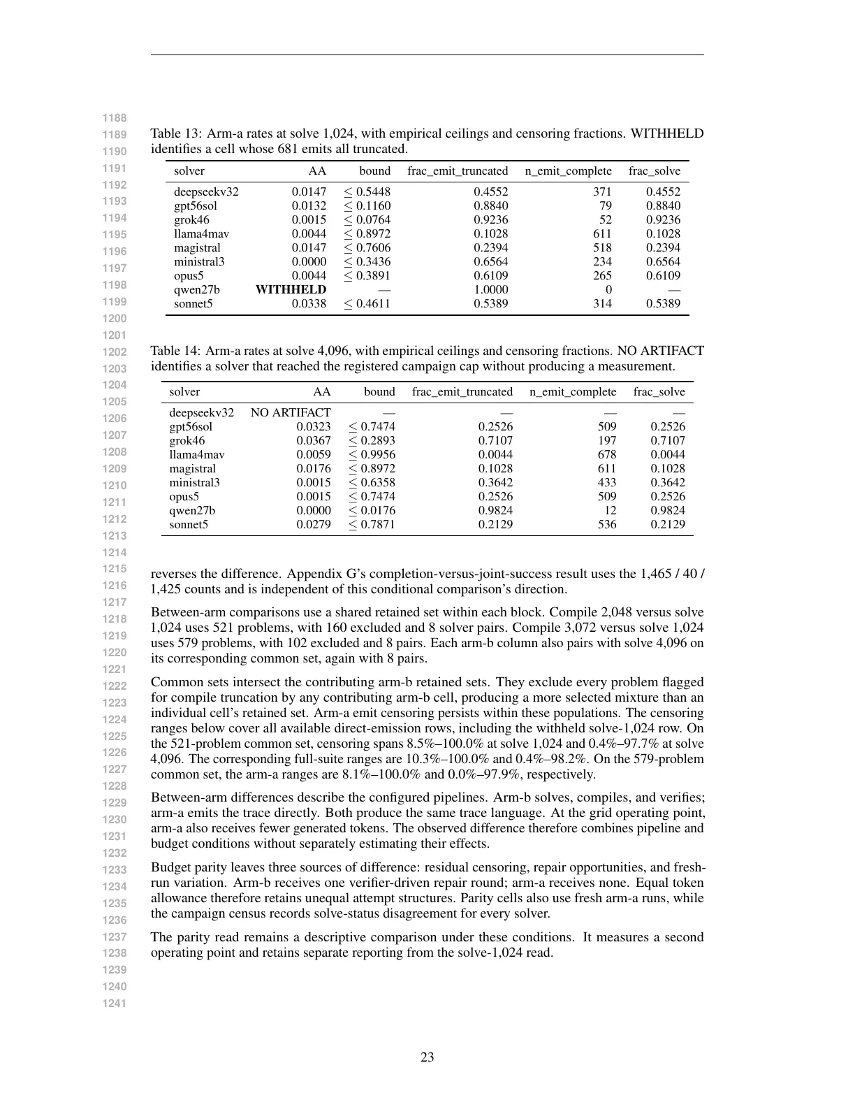
Text of page 23
Table 13: Arm-a rates at solve 1,024, with empirical ceilings and censoring fractions. WITHHELD
identifies a cell whose 681 emits all truncated.

solver

deepseekv32
gpt56sol
grok46
llama4mav
magistral
ministral3
opus5
qwen27b
sonnet5

AA

bound

frac_emit_truncated

n_emit_complete

frac_solve

0.0147
0.0132
0.0015
0.0044
0.0147
0.0000
0.0044
WITHHELD
0.0338

≤ 0.5448
≤ 0.1160
≤ 0.0764
≤ 0.8972
≤ 0.7606
≤ 0.3436
≤ 0.3891
—
≤ 0.4611

0.4552
0.8840
0.9236
0.1028
0.2394
0.6564
0.6109
1.0000
0.5389

371
79
52
611
518
234
265
0
314

0.4552
0.8840
0.9236
0.1028
0.2394
0.6564
0.6109
—
0.5389

Table 14: Arm-a rates at solve 4,096, with empirical ceilings and censoring fractions. NO ARTIFACT
identifies a solver that reached the registered campaign cap without producing a measurement.

solver

deepseekv32
gpt56sol
grok46
llama4mav
magistral
ministral3
opus5
qwen27b
sonnet5

AA

bound

frac_emit_truncated

n_emit_complete

frac_solve

NO ARTIFACT
0.0323
0.0367
0.0059
0.0176
0.0015
0.0015
0.0000
0.0279

—
≤ 0.7474
≤ 0.2893
≤ 0.9956
≤ 0.8972
≤ 0.6358
≤ 0.7474
≤ 0.0176
≤ 0.7871

—
0.2526
0.7107
0.0044
0.1028
0.3642
0.2526
0.9824
0.2129

—
509
197
678
611
433
509
12
536

—
0.2526
0.7107
0.0044
0.1028
0.3642
0.2526
0.9824
0.2129

reverses the difference. Appendix G’s completion-versus-joint-success result uses the 1,465 / 40 /
1,425 counts and is independent of this conditional comparison’s direction.

Between-arm comparisons use a shared retained set within each block. Compile 2,048 versus solve
1,024 uses 521 problems, with 160 excluded and 8 solver pairs. Compile 3,072 versus solve 1,024
uses 579 problems, with 102 excluded and 8 pairs. Each arm-b column also pairs with solve 4,096 on
its corresponding common set, again with 8 pairs.

Common sets intersect the contributing arm-b retained sets. They exclude every problem flagged
for compile truncation by any contributing arm-b cell, producing a more selected mixture than an
individual cell’s retained set. Arm-a emit censoring persists within these populations. The censoring
ranges below cover all available direct-emission rows, including the withheld solve-1,024 row. On
the 521-problem common set, censoring spans 8.5%–100.0% at solve 1,024 and 0.4%–97.7% at solve
4,096. The corresponding full-suite ranges are 10.3%–100.0% and 0.4%–98.2%. On the 579-problem
common set, the arm-a ranges are 8.1%–100.0% and 0.0%–97.9%, respectively.

Between-arm differences describe the configured pipelines. Arm-b solves, compiles, and verifies;
arm-a emits the trace directly. Both produce the same trace language. At the grid operating point,
arm-a also receives fewer generated tokens. The observed difference therefore combines pipeline and
budget conditions without separately estimating their effects.

Budget parity leaves three sources of difference: residual censoring, repair opportunities, and freshrun variation. Arm-b receives one verifier-driven repair round; arm-a receives none. Equal token
allowance therefore retains unequal attempt structures. Parity cells also use fresh arm-a runs, while
the campaign census records solve-status disagreement for every solver.

The parity read remains a descriptive comparison under these conditions. It measures a second
operating point and retains separate reporting from the solve-1,024 read.

23
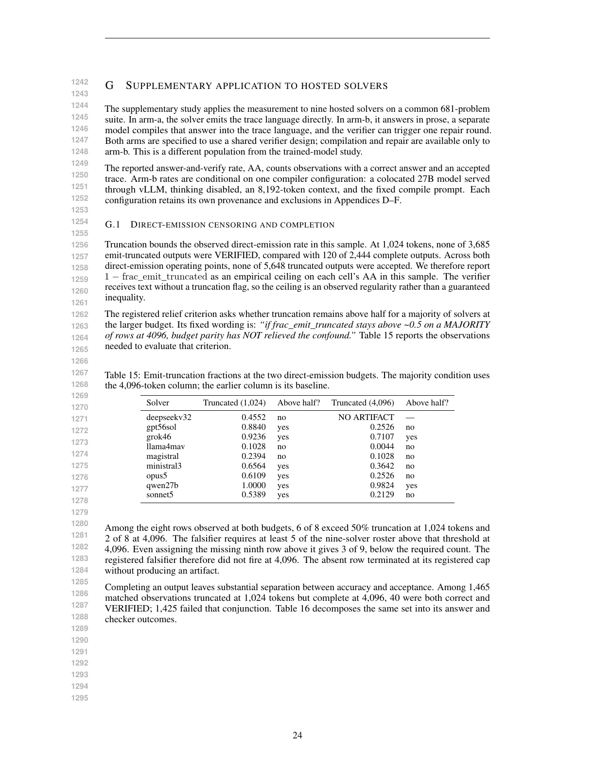
Text of page 24
G

The supplementary study applies the measurement to nine hosted solvers on a common 681-problem
suite. In arm-a, the solver emits the trace language directly. In arm-b, it answers in prose, a separate
model compiles that answer into the trace language, and the verifier can trigger one repair round.
Both arms are specified to use a shared verifier design; compilation and repair are available only to
arm-b. This is a different population from the trained-model study.

S UPPLEMENTARY APPLICATION TO HOSTED SOLVERS

The reported answer-and-verify rate, AA, counts observations with a correct answer and an accepted
trace. Arm-b rates are conditional on one compiler configuration: a colocated 27B model served
through vLLM, thinking disabled, an 8,192-token context, and the fixed compile prompt. Each
configuration retains its own provenance and exclusions in Appendices D–F.

G.1

D IRECT - EMISSION CENSORING AND COMPLETION

Truncation bounds the observed direct-emission rate in this sample. At 1,024 tokens, none of 3,685
emit-truncated outputs were VERIFIED, compared with 120 of 2,444 complete outputs. Across both
direct-emission operating points, none of 5,648 truncated outputs were accepted. We therefore report
1 − frac_emit_truncated as an empirical ceiling on each cell’s AA in this sample. The verifier
receives text without a truncation flag, so the ceiling is an observed regularity rather than a guaranteed
inequality.

The registered relief criterion asks whether truncation remains above half for a majority of solvers at
the larger budget. Its fixed wording is: “if frac_emit_truncated stays above ~0.5 on a MAJORITY
of rows at 4096, budget parity has NOT relieved the confound.” Table 15 reports the observations
needed to evaluate that criterion.

Table 15: Emit-truncation fractions at the two direct-emission budgets. The majority condition uses
the 4,096-token column; the earlier column is its baseline.

Solver

deepseekv32
gpt56sol
grok46
llama4mav
magistral
ministral3
opus5
qwen27b
sonnet5

Truncated (1,024)

0.4552
0.8840
0.9236
0.1028
0.2394
0.6564
0.6109
1.0000
0.5389

Above half?

no
yes
yes
no
no
yes
yes
yes
yes

Truncated (4,096)

NO ARTIFACT
0.2526
0.7107
0.0044
0.1028
0.3642
0.2526
0.9824
0.2129

Above half?

—
no
yes
no
no
no
no
yes
no

Among the eight rows observed at both budgets, 6 of 8 exceed 50% truncation at 1,024 tokens and
2 of 8 at 4,096. The falsifier requires at least 5 of the nine-solver roster above that threshold at
4,096. Even assigning the missing ninth row above it gives 3 of 9, below the required count. The
registered falsifier therefore did not fire at 4,096. The absent row terminated at its registered cap
without producing an artifact.

Completing an output leaves substantial separation between accuracy and acceptance. Among 1,465
matched observations truncated at 1,024 tokens but complete at 4,096, 40 were both correct and
VERIFIED; 1,425 failed that conjunction. Table 16 decomposes the same set into its answer and
checker outcomes.

24
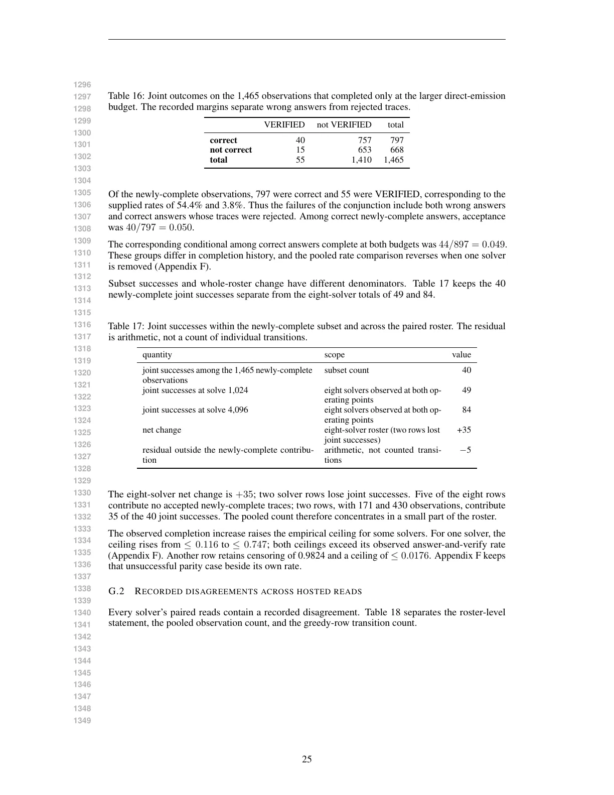
Text of page 25
Table 16: Joint outcomes on the 1,465 observations that completed only at the larger direct-emission
budget. The recorded margins separate wrong answers from rejected traces.

correct
not correct
total

not VERIFIED

total

40
15
55

757
653
1,410

797
668
1,465

Of the newly-complete observations, 797 were correct and 55 were VERIFIED, corresponding to the
supplied rates of 54.4% and 3.8%. Thus the failures of the conjunction include both wrong answers
and correct answers whose traces were rejected. Among correct newly-complete answers, acceptance
was 40/797 = 0.050.

The corresponding conditional among correct answers complete at both budgets was 44/897 = 0.049.
These groups differ in completion history, and the pooled rate comparison reverses when one solver
is removed (Appendix F).

Subset successes and whole-roster change have different denominators. Table 17 keeps the 40
newly-complete joint successes separate from the eight-solver totals of 49 and 84.

Table 17: Joint successes within the newly-complete subset and across the paired roster. The residual
is arithmetic, not a count of individual transitions.

VERIFIED

quantity

scope

joint successes among the 1,465 newly-complete
observations
joint successes at solve 1,024

subset count

40

eight solvers observed at both operating points
eight solvers observed at both operating points
eight-solver roster (two rows lost
joint successes)
arithmetic, not counted transitions

49

joint successes at solve 4,096

net change

residual outside the newly-complete contribution

value

84

+35

−5

The eight-solver net change is +35; two solver rows lose joint successes. Five of the eight rows
contribute no accepted newly-complete traces; two rows, with 171 and 430 observations, contribute
35 of the 40 joint successes. The pooled count therefore concentrates in a small part of the roster.

The observed completion increase raises the empirical ceiling for some solvers. For one solver, the
ceiling rises from ≤ 0.116 to ≤ 0.747; both ceilings exceed its observed answer-and-verify rate
(Appendix F). Another row retains censoring of 0.9824 and a ceiling of ≤ 0.0176. Appendix F keeps
that unsuccessful parity case beside its own rate.

G.2

R ECORDED DISAGREEMENTS ACROSS HOSTED READS

Every solver’s paired reads contain a recorded disagreement. Table 18 separates the roster-level
statement, the pooled observation count, and the greedy-row transition count.

25
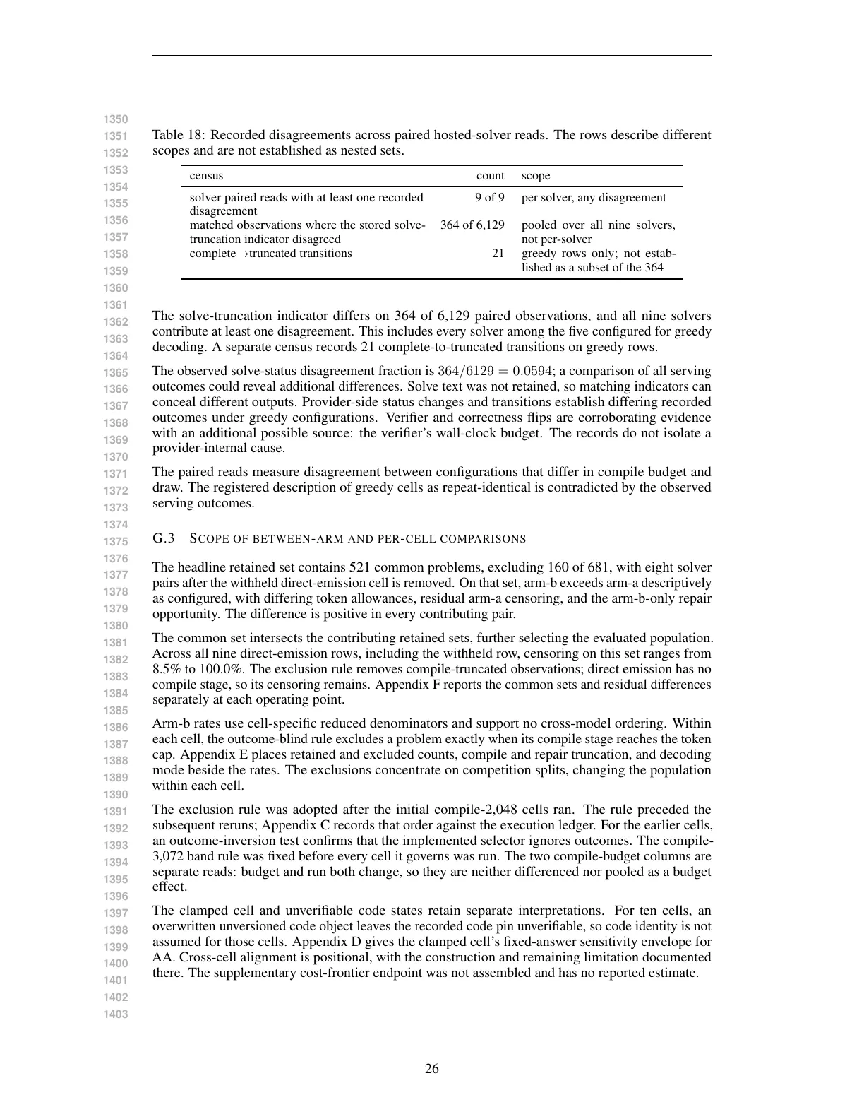
Text of page 26
Table 18: Recorded disagreements across paired hosted-solver reads. The rows describe different
scopes and are not established as nested sets.

census

count

scope

solver paired reads with at least one recorded
disagreement
matched observations where the stored solvetruncation indicator disagreed
complete→truncated transitions

9 of 9

per solver, any disagreement

364 of 6,129

21

pooled over all nine solvers,
not per-solver
greedy rows only; not established as a subset of the 364

The solve-truncation indicator differs on 364 of 6,129 paired observations, and all nine solvers
contribute at least one disagreement. This includes every solver among the five configured for greedy
decoding. A separate census records 21 complete-to-truncated transitions on greedy rows.

The observed solve-status disagreement fraction is 364/6129 = 0.0594; a comparison of all serving
outcomes could reveal additional differences. Solve text was not retained, so matching indicators can
conceal different outputs. Provider-side status changes and transitions establish differing recorded
outcomes under greedy configurations. Verifier and correctness flips are corroborating evidence
with an additional possible source: the verifier’s wall-clock budget. The records do not isolate a
provider-internal cause.

The paired reads measure disagreement between configurations that differ in compile budget and
draw. The registered description of greedy cells as repeat-identical is contradicted by the observed
serving outcomes.

G.3

S COPE OF BETWEEN - ARM AND PER - CELL COMPARISONS

The headline retained set contains 521 common problems, excluding 160 of 681, with eight solver
pairs after the withheld direct-emission cell is removed. On that set, arm-b exceeds arm-a descriptively
as configured, with differing token allowances, residual arm-a censoring, and the arm-b-only repair
opportunity. The difference is positive in every contributing pair.

The common set intersects the contributing retained sets, further selecting the evaluated population.
Across all nine direct-emission rows, including the withheld row, censoring on this set ranges from
8.5% to 100.0%. The exclusion rule removes compile-truncated observations; direct emission has no
compile stage, so its censoring remains. Appendix F reports the common sets and residual differences
separately at each operating point.

Arm-b rates use cell-specific reduced denominators and support no cross-model ordering. Within
each cell, the outcome-blind rule excludes a problem exactly when its compile stage reaches the token
cap. Appendix E places retained and excluded counts, compile and repair truncation, and decoding
mode beside the rates. The exclusions concentrate on competition splits, changing the population
within each cell.

The exclusion rule was adopted after the initial compile-2,048 cells ran. The rule preceded the
subsequent reruns; Appendix C records that order against the execution ledger. For the earlier cells,
an outcome-inversion test confirms that the implemented selector ignores outcomes. The compile-
3,072 band rule was fixed before every cell it governs was run. The two compile-budget columns are
separate reads: budget and run both change, so they are neither differenced nor pooled as a budget
effect.

The clamped cell and unverifiable code states retain separate interpretations. For ten cells, an
overwritten unversioned code object leaves the recorded code pin unverifiable, so code identity is not
assumed for those cells. Appendix D gives the clamped cell’s fixed-answer sensitivity envelope for
AA. Cross-cell alignment is positional, with the construction and remaining limitation documented
there. The supplementary cost-frontier endpoint was not assembled and has no reported estimate.

26